Review — An End-to-End Multi-Task Deep Learning Framework for Skin Lesion Analysis
Multi-Task Learning for Classification, Detection & Segmentation

An End-to-End Multi-Task Deep Learning Framework for Skin Lesion Analysis,
Song JBHI’20, by Tsinghua Shenzhen International Graduate School, University of British Columbia, and Shenzhen Institute of Future Media Technology,
2020 JBHI, Over 40 Citations (Sik-Ho Tsang @ Medium)
Medical Imaging, Medical Image Analysis, Multi-Task Learning
- An end-to-end multi-task deep learning framework is proposed for automatic skin lesion analysis.
- A loss function based on the focal loss and the jaccard distance is proposed.
Outline
- Dataset
- Skin Lesion Analysis Framework
- Loss Functions
- Experimental Results
1. Dataset


- The original dermoscopy images show a wide resolution range varying from 540×576 to 6688×6780. The major image size is around 2016×3024. The image is resized to 1024×1024 with zero padding.
- Zero-center normalization is performed on the resized images by subtracting pixel means in R, G, B channels separately.
- Five data augmentation operations are performed include flipping images horizontally and vertically, applying the affine transformation, multiplying each image with a random value between 0.8 and 1.5, and Gaussian blurring.
- The number of samples after data augmentation stays the same as that of the original training dataset (12666 benign samples, 1084 malignant samples).
2. Skin Lesion Analysis Framework

- The proposed model architecture consists of feature pyramid network (FPN), region proposal network (RPN) and three convolution subnets, where these subnets are used for classification, detection and segmentation separately.
2.1. ResNet Backbone
- ResNet is used as backbone, which takes the prepared 1024×1024 images as the inputs and the feature map size is reduced half when passed by every level. That is, the size of feature map in level 1 to 5 are 512×512, 256×256, 128×128, 64×64, 32×32, respectively.
2.2. Feature Pyramid Network (FPN)
- Then, a 1×1 convolution is performed on feature map in level 2 to 5 and denote as C2-C5. C5 is used as the top layer output of the FPN (P5), and after that, the second layer output (P4) is constructed by merging C4 and the feature map that up-samples P5 double.
- Similarly, the P3 and P2 can be gained in sequence.
- Finally, P2-P5 are taken after a 3×3 convolution as the FPN outputs and are fed into the next RPN.
2.3. Region Proposal Network (RPN)
- Inspired by Faster R-CNN, RPN is used for distinguishing foreground objects and background in dermoscopy images.
- Anchors are used to scan the image regions. Classification is performed to pick up the highest score bounding box that contains foreground objects.
- Then, positive and negative anchors are chosen according to the intersection-over-union (IOU) higher than 0.7, lower than 0.3, respectively.
- Proposals are acquired after applying non-maximum suppression (NMS).
2.4. Convolutional Subnets
- Feature pooling firstly to get the 7×7 fixed size of proposal feature map.
- Then, the pooled feature maps are fed into three convolution subnets separately.
- The Classify subnet is composed of two fully-connected layers and computes the probability towards a specific melanoma type based on the softmax (benign vs. malignant).
- The Detect subnet does bounding box regression to refine proposals aiming for more accurate localization.
- The Segment subnet uses the mask head proposed by Mask R-CNN to generate segmentation masks for each skin lesion. It consists of four convolution layers and one 2× up-sample layer and one sigmoid activation layer, where the sigmoid layer maps neuron values to binary mask form.
3. Loss Functions
3.1. RPN Loss with Focal Loss
- RPN classifies the foreground from all anchors and does the bounding box regression. The loss is composed of classification loss Lcls(pi, p∗i) and regression loss Lreg(ti, t∗i):
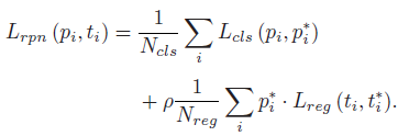
- where pi and ti stand for the prediction probability of anchor i being foreground and its estimated coordinates respectively, while p∗i and t∗i denote the corresponding ground truth information, and Ncls and Nreg are the number of anchors used for computing the classification loss Lcls(pi, p∗i) and the regression loss Lreg(ti, t∗i) respectively.
- ρ=10.
- In the skin lesion case, much less malignant samples can cause the network fail to learn melanoma features. Inspired by Focal loss in RetinaNet, the classification loss becomes:
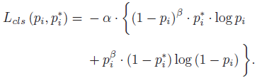
- where α=0.25, β=2. The benign lesions are dominant (pi is higher), so the corresponding weight (1 − pi)^β gets lower. Similarly, the probability of malignant lesions (1−pi) is lower and its weight (pi^β) gets higher.
- Such a loss function magnifies the effect of fewer positive samples.
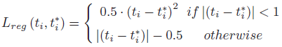
- The smooth L1 loss is adopted here to compute the regression loss due to its insensitivity to outliers:
3.2. Segmentation Loss
- The jaccard distance measures the dissimilarity between two sets and its complimentary jaccard index is an evaluation metric for medical image segmentation. It serves as a regularization term to improve the segmentation performance in addition to the binary cross entropy loss:
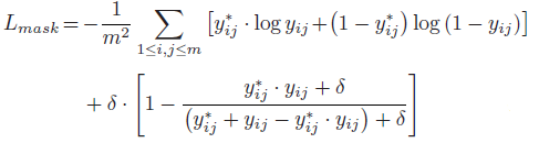
- δ=100.
3.3. Total Loss
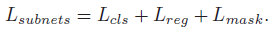
- The overall loss in the framework is defined as the sum of the RPN loss and the convolution subnets losses:
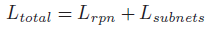
- where:
4. Experimental Results
4.1. Metrics
- For classification, the classification accuracy, the average precision (AP), the area under the ROC curve (AUC), the sensitivity (SE) and specificity (SP) are used to measure classification performances.
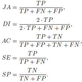
- For segmentation, there are five metrics suggested in ISIC 2017 challenge, including Jaccard index (JA), Dice coefficient (DI), pixel accuracy (AC), sensitivity (SE) and specificity (SP):
4.2. Classification Performance
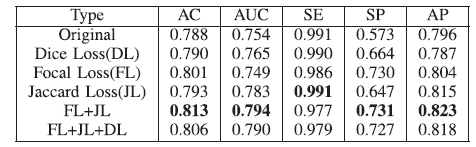
- With both focal loss (FL) and jaccard loss (JL), the best performance is obtained.
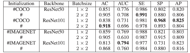
- A larger batch size yields a higher AC (but lower AUC and AP) when the initialization and backbone are the same.
- For example, if we choose the batch size 2×2 under COCO initialization and ResNet-50, AC increases from 0.851 to 0.905, AUC decreases from 0.776 to 0.708 and AP decreases from 0.820 to 0.806.

The proposed method achieves the highest AC 0.891, SE 0.996, SP 0.723, AP 0.815 among all methods. In terms of AC, SP and AP, there is a huge performance gain that demonstrates the effectiveness of the proposed framework in handling such a class imbalance dataset.
4.2. Segmentation Performance
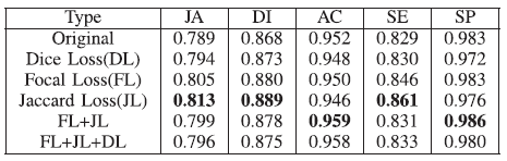
- When compared with the original loss function (cross entropy), in terms of JA, DI and SE metrics, FL, JL and FL+JL all yield higher values.
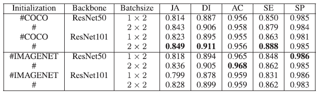
- With the setting (the COCO initialization, ResNet-101, batch size 2×2), the highest segmentation performance is obtained, i.e., JA 0.849, DI 0.911 and SE 0.888.
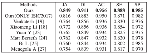
The proposed framework yields the best results in terms of all studied metrics. In terms of JA and DI (the main ranking metrics for ISIC 2017 challenge), a significant performance gain is noted, exceeding nearly six points than state-of-the-art methods.
4.3. Multi-Task Learning Study

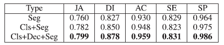
Both classification and segmentation results in the multi-task setting are better than that in the single task setting.
4.4. Visualizations
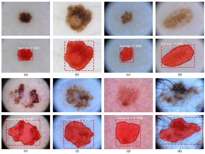
- (c), (d), (g) show obscure boundary and poor illumination.
- (e), (f), (h) show the irregular shape of melanoma. In addition, strong hair artifacts are shown in (h).
- Moreover, the malignant skin lesions are hard to classify because of the inadequate samples.
Authors mention that attention mechanism, dilated convolution and group normalization will be explored in the future.
Reference
[2020 JBHI] [Song JBHI’20]
An End-to-End Multi-Task Deep Learning Framework for Skin Lesion Analysis
4.3. Biomedical Image Multi-Task Learning
2018 … 2020 [Song JBHI’20] … 2021 [Ciga JMEDIA’21]
