Review — Label Propagation for Deep Semi-supervised Learning

Assign Pseudo Labels to Unlabeled Data Using Label Propagation

Label propagation on manifolds toy example. Triangles denote labeled, and circles unlabeled training data, respectively. Left: color-coded ground truth for labeled points, and gray color for unlabeled points. Right: color-coded pseudo-labels inferred by diffusion that are used to train the CNN.

Label Propagation for Deep Semi-supervised Learning
Label Propagation, by Czech Technical University in Prague, and Univ Rennes
2019 CVPR, Over 200 Citations (Sik-Ho Tsang @ Medium)
Semi-Supervised Learning, Pseudo Label, Image Classification

• A new iterative process is proposed, in which a transductive label propagation method is employed that is based on the manifold assumption to make predictions on the entire dataset.
• These predictions are used to generate pseudo-labels for the unlabeled data and train a deep neural network.

Outline

1. Label Propagation
2. Experimental Results

1. Label Propagation

Label Propagation Overview

1.1. Overview

• Step 1: Starting from a randomly initialized network, the network is trained in a supervised fashion on the labeled examples:

• where XL and YL are inputs and labels of labeled data. Cross entropy loss is used for ls. fθ is the neural network with parameters θ.
• Step 2: Then an iterative process is initiated where at each iteration a nearest neighbor graph of the entire training set in the feature space of the current network is computed, labels are propagated by transductive learning, and then the network is trained on the entire training set, with true labels or pseudo-labels on the labeled or unlabeled examples respectively, where the pseudo-labels are weighted per example and per class according to prediction certainty and inverse class population, respectively. (More details in 1.2.)

1.2. Iterative Process with Label Propagation

Iterative Process with Label Propagation

1.2.1. Label Propagation

Unlike some other semi-supervised learning approach that uses a pretrained network to predict the (hard or soft) pseudo labels, the method in this paper uses the image representation vector (descriptor) obtained just before the last fully connected layer, to propagate the labels as pseudo labels.

• Given a network with parameters θ, the descriptor set V is constructed:

• where Φθ is the network before fully connected layer and softmax.
• A sparse affinity matrix A ∈ R^(n×n) with elements is computed:

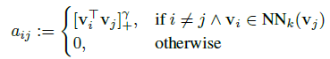
• where NNk denotes the set of k nearest neighbors in X, and γ is a parameter following recent work on manifold-based search [20].
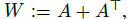
• Then, let W as a symmetric nonnegative adjacency matrix with zero diagonal:

• Further, the conjugate gradient (CG) method is used to solve linear system:

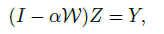
• where α ∈ [0, 1) is a parameter. Finally, the pseudo-labels are inferred:

• where ^yi is given by:

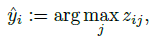
• where zij is the (i, j) element of matrix Z.

1.2.2. Weighted Pseudo Labels

• Each pseudo-label is associated with a weight reflecting the certainty of the prediction.
• Entropy is used as a measure of uncertainty, to assign weight ωi to example xi, defined by:

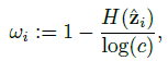
• Thus, higher entropy, lower certainty, and consequently lower weight ωi, and vice versa.
• For class imbalance issue, the weight ζj is assigned class j that is inversely proportional to class population, defined as:

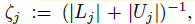
• where Lj (resp. Uj) are the examples labeled (resp. pseudo-labeled) as class j.
• Given the above definitions of per-example and per-class weights, the following weighted loss is associated to the labeled and pseudo-labeled examples:

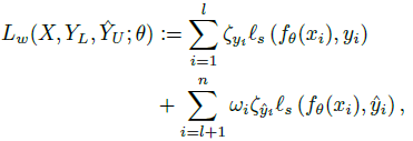
• which is the sum of weighted versions of Ls and Lp. (Ls is the supervised loss using labeled data and Lp is the supervised loss using pseudo labeled data.)

2. Experimental Results

• Mini-batch size B=BU+BL, where BL images are labeled and BU images are originally unlabeled. BL=50 for CIFAR-10 and BL=31 for CIFAR100 and Mini-ImageNet. Same is also applied for Mean Teacher (MT).
• One epoch is defined as one pass through all originally unlabeled examples in the training set, meaning that images in IL appear multiple times per epoch.
• The same diffusion parameters as [20]. k=50 for graph construction, γ=3 and α=0.99.
• ωi and ζj are updated after each epoch.

2.1. CIFAR-10

Error rate versus number of labeled images on CIFAR-10 using different methods.

Comparison with the state of the art on CIFAR-10

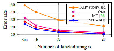
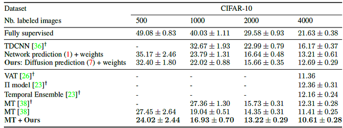
• “13-layer” network is used as in MT.
• Only 500 labeled examples are used for training and the rest of the training set is considered unlabeled.

MT+proposed label propagation obtained the the lowest error rates. The benefit is larger when the number of labels is reduced.

• It is also shown that label propagation is complementary to unsupervised loss, such as the one used by MT.

2.2. CIFAR-100 and Mini-ImageNet

Performance comparison on CIFAR-100 and Mini-ImageNet with 4k and 10k labeled images

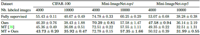
• “13-layer” network is used as in Mean Teacher (MT) for CIFAR-100.
• ResNet-18 is used for Mini-ImageNet.

The same holds for CIFAR-100 and Mini-ImageNet for 10k available labels.

• Label propagation also achieves a lower error rate than temporal ensemble (38.65%) and Π-model (39:19%) on CIFAR-100 with 10k labels.
• On Mini-ImageNet with 4k available labels, the best performance is achieved when using label propagation without combining with MT.

Reference

[2019 CVPR] [Label Propagation]
Label Propagation for Deep Semi-supervised Learning

Weakly/Semi-Supervised Learning

2013 [Pseudo-Label (PL)] 2017 [Mean Teacher] 2018 [WSL] 2019 [Billion-Scale] [Label Propagation]

My Other Previous Paper Readings