Review — t-SNE: Visualizing Data using t-SNE (Data Visualization)

Visualizing High-Dimensional Data in Low-Dimensional Space

8 min readJan 31, 2021

**t-SNE on MNIST Data set (From Google TechTalk by the First Author, Laurens van der Maaten,** https://www.youtube.com/watch?v=RJVL80Gg3lA)

In this story, Visualizing Data using t-SNE, t-SNE, by Tilburg University, and University of Toronto, is briefly reviewed. It is a very famous paper by Prof. Hinton. In this paper:

t-SNE is proposed, compared to SNE, it is much easier to optimize.
t-SNE reduces the crowding problem, compared to SNE.
t-SNE has been used in various fields for data visualization.

This is a paper in 2008 JMLR with over 17000 citations. (Sik-Ho Tsang @ Medium) It was also presented in 2013 Google TechTalk by author.

Outline

Dimensionality Reduction for Data Visualization
Brief Review of SNE
t-Distributed Stochastic Neighbor Embedding (t-SNE)
Experimental Results
More Results in Google TechTalk

1. Dimensionality Reduction for Data Visualization

Suppose we have high-dimensional data set X = {x1, x2, …, xn}, and we want to reduce the dimension into two or three-dimensional data Y = {y1, y2, …, yn} that can be displayed in a scatterplot.
In the paper, the low-dimensional data representation Y is referred as a map, and to the low-dimensional representations yi of individual data points as map points.

The aim of dimensionality reduction is to preserve as much of the significant structure of the high-dimensional data as possible in the low-dimensional map.

Linear mapping, such as PCA, cannot perform well.
t-SNE is proposed for mapping the high-dimensional data set X to low-dimensional data representation Y, while preserving the high-dimensional data structure.

2. Brief Review of SNE

2.1. SNE

Stochastic Neighbor Embedding (SNE) starts by converting the high-dimensional Euclidean distances between datapoints into conditional probabilities that represent similarities.

The similarity of datapoint xj to datapoint xi is the conditional probability, pj|i, that xi would pick xj as its neighbor if neighbors were picked in proportion to their probability density under a Gaussian centered at xi.

For nearby datapoints, pj|i is relatively high, whereas for widely separated datapoints, pj|i will be almost infinitesimal.
Mathematically, the conditional probability pj|i is:

where σi is the variance of the Gaussian that is centered on datapoint xi.
The similarity of map point yj to map point yi is modelled by:

SNE aims to find a low-dimensional data representation that minimizes the mismatch between pj|i and qj|i.
SNE minimizes the sum of Kullback-Leibler divergences over all datapoints using a gradient descent method. The cost function C is given by:

in which Pi represents the conditional probability distribution over all other datapoints given datapoint xi, and Qi represents the conditional probability distribution over all other map points given map point yi.
In particular, there is a large cost for using widely separated map points to represent nearby datapoints (i.e., for using a small qj|i to model a large pj|i), but there is only a small cost for using nearby map points to represent widely separated datapoints.
In other words, the SNE cost function focuses on retaining the local structure of the data in the map.

2.2. Selection of σi

In dense regions, a smaller value of σi is usually more appropriate than in sparser regions. SNE performs a binary search for the value of σi that produces a Pi with a fixed perplexity that is specified by the user. The perplexity is defined as:

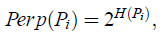
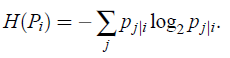
where H(Pi) is the Shannon entropy of Pi:

2.3. Gradient Descent

The minimization of the cost function C is performed using a gradient descent method:

Physically, the gradient may be interpreted as the resultant force created by a set of springs between the map point yi and all other map points yj.
The spring between yi and yj repels or attracts the map points depending on the distance.
The force exerted by the spring between yi and yj is proportional to its length, and also proportional to its stiffness, which is the mismatch (pj|i-qj|i+pi|j-qi|j) between the pairwise similarities of the data points and the map points.
The gradient descent is initialized by sampling map points randomly from an isotropic Gaussian with small variance that is centered around the origin.
To avoid poor local minima, a relatively large momentum term is added to the gradient. The gradient update with a momentum term is given by:

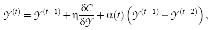
where Y(t) indicates the solution at iteration t, η indicates the learning rate, and α(t) represents the momentum at iteration t.
(More details can be found in the paper.)

3. t-Distributed Stochastic Neighbor Embedding (t-SNE)

So, what’s new in t-SNE? t-SNE solves the “crowding problem” originally in SNE.
t-SNE is capable of capturing much of the local structure of the high-dimensional data very well, while also revealing global structure such as the presence of clusters at several scales.
The cost function used by t-SNE differs from the one used by SNE in two ways:

It uses a symmetrized version of the SNE cost function with simpler gradients.
It uses a Student-t distribution rather than a Gaussian to compute the similarity between two points in the low-dimensional space. t-SNE employs a heavy-tailed distribution in the low-dimensional space to alleviate both the crowding problem and the optimization problems of SNE.

3.1. Symmetric SNE

Symmetric SNE minimizes a single Kullback-Leibler divergence between a joint probability distribution, P, in the high-dimensional space and a joint probability distribution, Q, in the low-dimensional space:

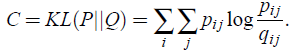
With pij=pji and qij=qji.

Therefore, no matter the data points i and j are close to each other or far away from each other, when the mapping is good enough, pij is close to qij, pij/qij is close to 1.
Taking the log, log(pij/qij) is close to 0, the cost for that i and j is 0.
If all the points mapped correctly, the total cost C will be small.

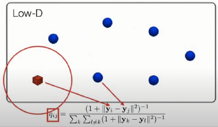
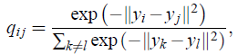
pairwise similarities in the low-dimensional map *qij*

In symmetric SNE, the pairwise similarities in the low-dimensional map qij are given by (also as shove above):

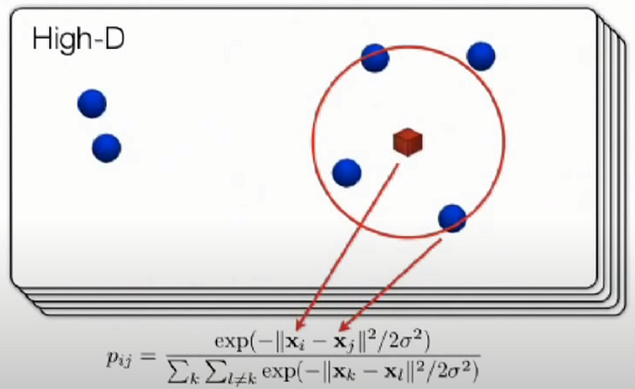
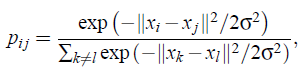
Pairwise similarities in the high-dimensional space *pij*

And the pairwise similarities in the high-dimensional space pij is given by (also as shove above):

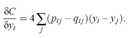
The gradient of symmetric SNE is fairly similar to that of asymmetric SNE, and is given by:

It is observed that symmetric SNE seems to produce maps that are just as good as asymmetric SNE, and sometimes even a little better.

3.2. The Crowding Problem

For instance, in 10 dimensions, it is possible to have 11 datapoints that are mutually equidistant and there is no way to model this faithfully in a two-dimensional map.
So if the datapoints are approximately uniformly distributed in the region around i on the 10-dimensional manifold, and we try to model the distances from i to the other datapoints in the 2-dimensional map, we get the following “crowding problem”.
The area of the 2-dimensional map is not large enough to accommodate 11 datapoints.
To solve this, in the low-dimensional map, we can use a probability distribution that has much heavier tails than a Gaussian to convert distances into probabilities.
This allows a moderate distance in the high-dimensional space to be faithfully modeled by a much larger distance in the map and, as a result, it eliminates the unwanted attractive forces between map points that represent moderately dissimilar datapoints.
In t-SNE, a Student t-distribution with one degree of freedom (which is the same as a Cauchy distribution) is employed as the heavy-tailed distribution in the low-dimensional map.
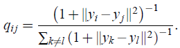
Using this distribution, the joint probabilities qij are defined as:

When heavy-tailed distribution, the distance of the points in the lower dimensional space is larger compared to when the tails are normally distributed.

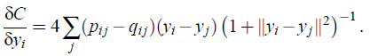
The gradient of the Kullback-Leibler divergence between P and the Student-t based joint probability distribution Q becomes:

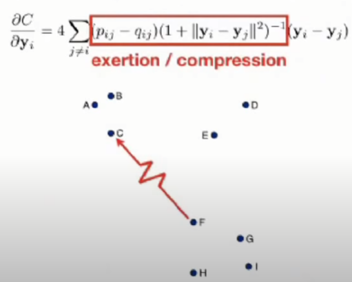
The gradient can be interpreted as the repelling or attracting force.

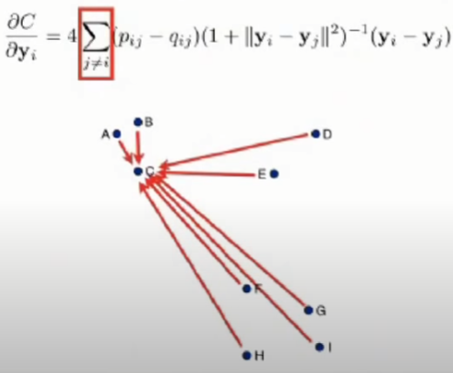
And the summation is the total force of all datapoints.
(There are still many details not yet mentioned here. If interested, please feel free to read the paper.)

4. Experimental Results

In all experiments, PCA is used to reduce the dimensionality of the data to 30 first. This speeds up the computation of pairwise distances between the datapoints and suppresses some noise without severely distorting the interpoint distances.
Then , the 30-dimensional representation is reduced to a two-dimensional map using t-SNE and the resulting map is shown as a scatterplot.

**Visualizations of the MNIST data set using t-SNE**

The map produced by t-SNE contains some points that are clustered with the wrong class, but most of these points correspond to distorted digits many of which are difficult to identify.

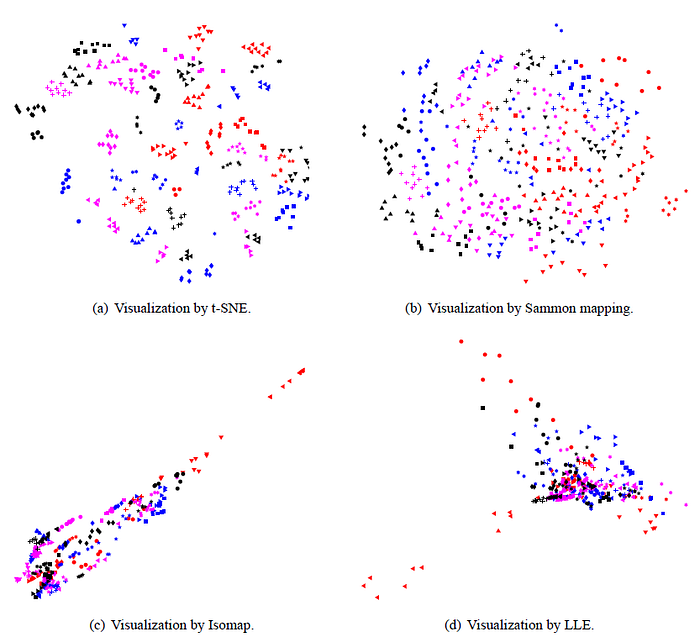
**Visualizations of the Olivetti faces data set**

Comparatively, Isomap and LLE produce solutions that provide little insight.

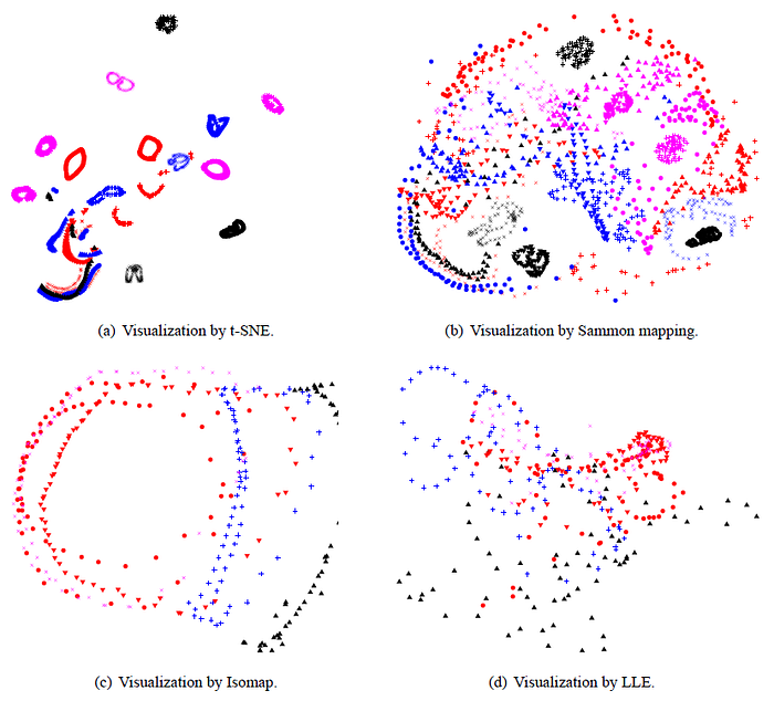
**Visualizations of the COIL-20 data set**

For many of the 20 objects, t-SNE accurately represents the one-dimensional manifold of viewpoints as a closed loop.
(Again, there are large portions of paragraphs for the experiments that hasn’t shown here, please feel free to read the paper if interested.)

5. More Results in Google TechTalk

In 2013, the first author, Laurens van der Maaten, presented t-SNE in Google TechTalk.
(It is crazily amazing that t-SNE was published in 2008, it was presented in Google TechTalk in 2013, while it is still useful right now !!)