Review: Representation Learning with Contrastive Predictive Coding (CPC/CPCv1)
Representation Learning Using InfoNCE Loss

In this story, Representation Learning with Contrastive Predictive Coding, (CPC/CPCv1), by DeepMind, is reviewed. In this paper:
- Contrastive Predictive Coding (CPC) is proposed, which is a universal unsupervised learning approach to extract useful representations from high-dimensional data.
- A noise-Contrastive Estimation Loss, namely InfoNCE Loss, is used, which induces the latent space to capture information that is maximally useful to predict future samples.
- Four distinct domains are used for evaluation: speech, images, text and reinforcement learning in 3D environments.
This is a paper in 2018 arXiv with over 1800 citations. (Sik-Ho Tsang @ Medium) This paper makes use of NCE and Negative Sampling in NLP for representation learning/self-supervised learning.
Outline
- Motivation and Intuition of Contrastive Predictive Coding (CPC)
- Contrastive Predictive Coding (CPC): Overview
- InfoNCE Loss and Mutual Information Estimation
- Experiments for Audio
- Experiments for Vision
- Experiments for Natural Language
- Experiments for Reinforcement Learning
1. Motivation and Intuition of Contrastive Predictive Coding (CPC)
- Unimodal losses such as means squared error and cross-entropy are not very useful, modeling p(x|c) directly may not be optimal, where target x (future) and context c (present).
- For example, images may contain thousands of bits of information while the high-level latent variables such as the class label contain much less information (10 bits for 1,024 categories).
- However, unsupervised learning is yet to see a breakthrough as well.
- Predictive coding has been used for long time in data compression.
- The main intuition of the model is to learn the representations that encode the underlying shared information between different parts of the (high-dimensional) signal. At the same time it discards low-level information and noise that is more local.
- When predicting future information, CPC instead encode the target x (future) and context c (present) into a compact distributed vector representations in a way that maximally preserves the mutual information of the original signals x and c defined as:

2. Contrastive Predictive Coding (CPC): Overview
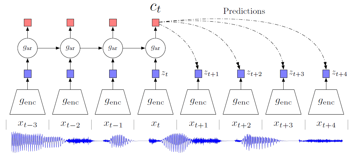
- genc: First, a non-linear encoder genc maps the input sequence of observations xt to a sequence of latent representations zt = genc(xt), potentially with a lower temporal resolution.
- gar: Next, an autoregressive model gar summarizes all z⩽t in the latent space and produces a context latent representation ct = gar(z⩽t).
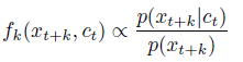
As argued in the previous section, we do not predict future observations xt+k directly with a generative model pk(xt+k|ct). Instead we model a density ratio which preserves the mutual information between xt+k and ct:
- The density ratio f can be unnormalized.
- A simple log-bilinear model can be used:
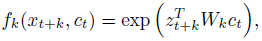
A linear transformation WTk ct is used for the prediction with a different Wk for every step k.
- Although p(x) or p(x|c) cannot be evaluated directly, samples from these distributions can be utilized such as by Noise-Contrastive Estimation (NCE).
In the proposed model, either of zt and ct could be used as representation for downstream tasks.
3. InfoNCE Loss and Mutual Information Estimation
- Both the encoder and autoregressive model are trained to jointly optimize a loss based on NCE, called InfoNCE.
- Given a set X = {x1, …, xN} of N random samples containing one positive sample from p(xt+k|ct) and N-1 negative samples from the ‘proposal’ distribution p(xt+k)

- Recall in the previous section that:
- Optimizing this loss will result in fk(xt+k, ct) estimating the density ratio mentioned in the previous section.
- The optimal probability for this loss is written as p(d=i|X, ct) with [d=i] being the indicator that sample xi is the ‘positive’ sample.
- The probability that sample xi was drawn from the conditional distribution p(xt+k|ct) rather than the proposal distribution p(xt+k) can be derived as follows:
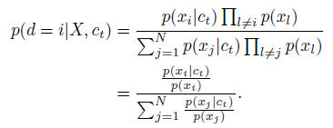
- As seen, the optimal value for f(xt+k, ct) is independent of the the choice of the number of negative samples N-1.
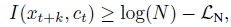
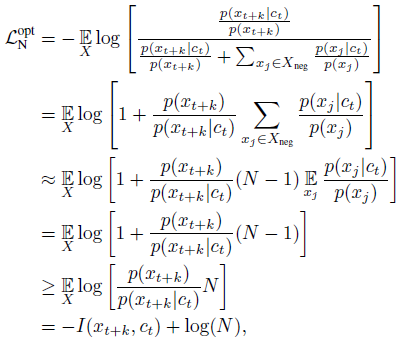
- Minimizing the InfoNCE loss Ln, is actually maximizing a lower bound on the mutual information I(xt+k, ct):
- The proof (By splitting X into the positive example and the negative examples Xneg):
- (InfoNCE loss is highly related to NCE & Negative Sampling used in NLP. Please feel free to read it if interested.)
4. Experiments for Audio
4.1. Pretext Task
- A 100-hour subset of the publicly available LibriSpeech dataset is used which does not have labels, but only raw text.
- Authors have made the aligned phone labels and our train/test split. The dataset contains speech from 251 different speakers.
- genc: The encoder architecture genc used in our experiments consists of a strided CNN that runs directly on the 16KHz PCM audio waveform. Five convolutional layers with strides [5, 4, 2, 2, 2], filter-sizes [10, 8, 4, 4, 4] and 512 hidden units with ReLU activations, are used.
- There is a feature vector for every 10ms of speech.
- gar: A GRU RNN for the autoregressive part of the model, gar with 256 dimensional hidden state. The output of the GRU at every timestep is used as the context c.
- A minibatch of 8 examples from which the negative samples in the contrastive loss are drawn.
12 timesteps in the future are predicted using the contrastive loss.
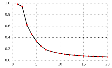
- The prediction task becomes harder as the target is further away.
4.2. Downstream Task
- To understand the representations extracted by CPC, the phone prediction performance is measured with a linear classifier trained on top of these features.
- The outputs of the GRU (256 dimensional) are extracted as, ct.
- A multi-class linear logistic regression classifier is trained.
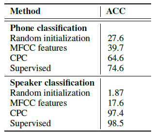
- Three baselines: Random initialized model (i.e., genc and gar areuntrained), MFCC features, and a model that is trained end-to-end supervised with the labeled data.
For phone classification, CPC obtains 64.6% accuracy.
When a single hidden layer is used instead, the accuracy increases from 64.6% to 72.5%, which is closer to the accuracy of the fully supervised model.
Interestingly, CPCs capture both speaker identity and speech contents, as demonstrated by the good accuracies attained with a simple linear classifier, which also gets close to the oracle, fully supervised networks.
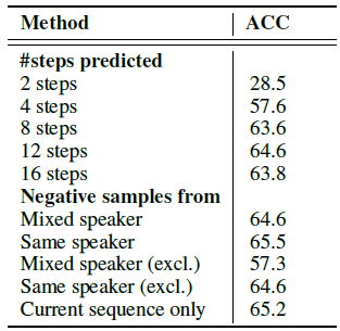
- Some other ablation experiments are also performed, i.e. how many steps to predict, predicting 12 steps obtains the best CPC representations.
- Also, where the negative samples are drawn from (this part, all are to predcit 12 steps) are also tested. (excl. means excluding negative samples from the current sequence.) It is found that negative samples drawn from the same speaker obtains the best CPC representations.
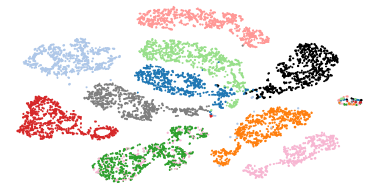
- t-SNE visualization shows how discriminative the embeddings are for speaker voice-characteristics.
5. Experiments for Vision
5.1. Pretext Task
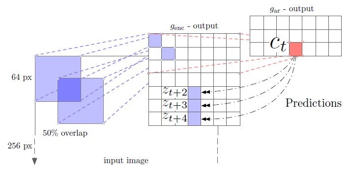
- genc: A ResNet v2 101 architecture is used as the image encoder genc to extract CPC representations.
- After unsupervised training, a linear layer is trained to measure classification accuracy on ImageNet labels.
- For each of the 64×64 crops, a 60×60 subcrop is picked and padded them back to a 64×64 image. Each crop is then encoded by the ResNet-v2–101 encoder. The outputs from the third residual block, are used to spatially mean-pool to get a single 1024-d vector per 64×64 patch.
- For each image, this results in a 7×7×1024 tensor.
- gar: A PixelCNN-style autoregressive model (An image generation method) is used to make predictions about the latent activations in following rows top-to-bottom, predict up to five rows from the 7×7 grid.
- The contrastive loss is applied for each patch in the row.
5.2. Downstream Task
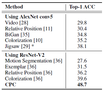
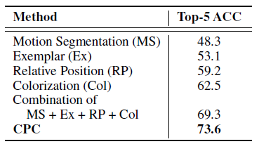
- CPC outperforms Context Prediction, Colorization, Jigsaw Puzzles, BiGAN, etc.
Despite being relatively domain agnostic, CPCs improve upon state-of-the-art by 9% absolute in top-1 accuracy, and 4% absolute in top-5 accuracy.
6. Experiments for Natural Language
6.1. Pretext Task
- CPC follows closely the procedure from Skip-Thought vectors model, first learn the unsupervised model on the BookCorpus dataset.
- (Please feel free to read Skip-Thought vectors if interested.)
- genc & gar: The model consists of a simple sentence encoder genc (a 1D-convolution + ReLU + mean-pooling) that embeds a whole sentence into a 2400-dimension vector z, followed by a GRU (2400 hidden units) as gar which predicts up to 3 future sentence embeddings with the contrastive loss to form c.
6.2. Downstream Task
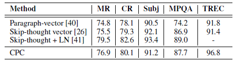
- For the classification tasks, the following datasets are used: movie review sentiment (MR) [43], customer product reviews (CR) [44], subjectivity/objectivity [45], opinion polarity (MPQA) [46] and question-type classification (TREC) [47].
- A logistic regression classifier is trained.
The performance of our method is very similar to the Skip-Thought vector model [26], with the advantage that it does not require a powerful LSTM as word-level decoder, therefore much faster to train.
6. Experiments for Reinforcement Learning

- 5 reinforcement learning in 3D environments of DeepMind Lab [51] are tested: rooms_watermaze, explore_goal_locations_small, seekavoid_arena_01, lasertag_three_opponents_small and rooms_keys_doors_puzzle.
- The standard batched A2C [52] agent is used as base model.
- CPC is used as an auxiliary loss, this setting is different from the one in audio, text, and images.
- The unroll length for the A2C is 100 steps and we predict up to 30 steps in the future to derive the contrastive loss.
- For 4 out of the 5 games, performance of the agent improves significantly with the contrastive loss after training on 1 billion frames.
- (I am not familiar with reinforcement learning, if interested, please feel free to read the paper.)
Later on, CPCv2 is published in 2020 ICLR, hope I have time to review it in the coming future.
Reference
[2018 arXiv] [CPC/CPCv1]
Representation Learning with Contrastive Predictive Coding
Self-Supervised Learning
2008–2010 [Stacked Denoising Autoencoders] 2014 [Exemplar-CNN] 2015 [Context Prediction] 2016 [Context Encoders] [Colorization] [Jigsaw Puzzles] 2017 [L³-Net] [Split-Brain Auto] [Mean Teacher] 2018 [RotNet/Image Rotations] [DeepCluster] [CPC/CPCv1]