Review — YOLOv12: Attention-Centric Real-Time Object Detectors

YOLOv12: Attention-Centric Real-Time Object Detectors
YOLOv12, by University at Buffalo, and University of Chinese Academy of Sciences
2025 arXiv v1 (Sik-Ho Tsang @ Medium)Object Detection
2014 … 2023 [YOLOv7] [YOLOv8] [Lite DETR] [YOLOv8 for Helmet Violation Detection] [YOLOv8 for Flying Object Detection] 2024 [YOLOv9] [YOLOv10] [RT-DETR]
==== My Other Paper Readings Are Also Over Here ====
- (Sorry that it’s been a long time that I haven’t updated the Medium while I am busy on my new job. Also, right now, everybody uses LLM, such as OpenAI o3 and DeepSeek for summarizing the paper for reading. I wonder if it is still valuable for writing the tech blog article.)
- In brief, YOLOv12 introduces Area Attention, and also R-ELAN for better performance.
- Let’s dive in!
Outline
- YOLOv12
- Results
1. YOLOv12
1.1. Preliminaries
- The attention mechanism is inherently slower than convolution neural networks (CNN) due to two factors:
- Complexity. First, the computational complexity of the self-attention operation scales quadratically with the input sequence length L. Moreover, another significant factor is that most attention-based vision transformers, due to their complex designs (e.g., window partitioning/reversing in Swin transformer [39]) and the introduction of additional modules (e.g., positional encoding), gradually accumulate speed overhead.
- Computation. Second, in the attention computation process, memory access patterns are less efficient compared to CNNs, such as the attention map and the softmax map. Additionally, irregular memory access patterns in attention introduce further latency compared to CNNs.
1.2. Area Attention

The simple yet efficient area attention module is proposed. As illustrated in Figure 2 (rightmost), the feature map with the resolution of (H, W) is divided into l segments of size (H/l, W) or (H, W/l).
The default value of l is set to 4, reducing the receptive field to 1/4 of the original, yet it still maintains a large receptive field.
1.3. Residual Efficient Layer Aggregation Networks (R-ELAN)

- As shown in Figure 3 (b), ELAN splits the output of a transition layer (a 1×1 convolution), processes one split through multiple modules, then concatenates the all the outputs and applies another transition layer (a 1 × 1 convolution) to align dimensions. However, as analyzed by [57], this architecture can introduce instability. Authors argue that such a design causes gradient blocking and lacks residual connections from input to output.
A new aggregation approach is proposed in Figure 3 (d). A residual shortcut is introduced from input to output throughout the block with a scaling factor (default to 0.01).
The proposed design applies a transition layer to adjust the channel dimensions and produces a single feature map. This feature map is then processed through subsequent blocks followed by the concatenation, forming a bottleneck structure.
- This approach not only preserves the original feature integration capability, but also reduces both computational cost and parameter / memory usage.
1.4. Architectural Improvements
- The hierarchical design of the previous YOLO systems is retained.
- The design of stacking three blocks in the last stage of the backbone is removed, only a single R-ELAN block is retained.
- The first two stages of the backbone from YOLOv11 [28] is retained.
- The MLP ratio is adjusted from 4 to 1.2 (or 2 for the N- / S- / M-scale models) is used to better allocate computational resources for better performance.
- Adopting nn.Conv2d+BN instead of nn.Linear+LN to fully exploit the efficiency of convolution operators
- Removing positional encoding, and introducing a large separable convolution (7×7).
- etc.
1.5. Model Variants
The YOLOv12 family includes 5 variants: YOLOv12-N, YOLOv12-S, YOLOv12-M, YOLOv12-L, and YOLOv12-X.
- All models are trained for 600 epochs using the SGD optimizer.
2. Results
2.1. SOTA Comparisons

e.g.: For N-scale models, YOLOv12-N outperforms YOLOv6–3.0-N [32], YOLOv8-N [58], YOLOv10-N [53], and YOLOv11 [28] by 3.6%, 3.3%, 2.1%, and 1.2% in mAP, respectively, while maintaining similar or even fewer computations and parameters, and achieving the fast latency speed of 1.64 ms/image.
- For S-scale models, YOLOv12-S, with 21.4G FLOPs and 9.3M parameters, achieves 48.0 mAP with 2.61 ms/image latency. It outperforms YOLOv8-S [24], YOLOv9-S [58], YOLOv10-S [53], and YOLOv11-S [28] by 3.0%, 1.2%, 1.7%, and 1.1%, respectively, while maintaining similar or fewer computations.
- For M-scale models, YOLOv12-M, with 67.5G FLOPs and 20.2M parameters, achieves 52.5 mAP performance and 4.86 ms/image speed.
- For L-scale models, YOLOv12-L even surpasses YOLOv10-L [53] with 31.4G fewer FLOPs.
- For X-scale models, YOLOv12-X significantly outperforms YOLOv10-X [53] / YOLOv11-X [28] by 0.8% and 0.6%, respectively, with comparable speed, FLOPs, and parameters.
2.2. Speed Comparison
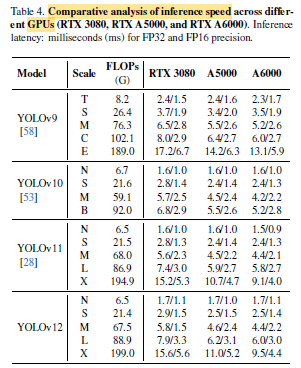
YOLOv12 achieves a significantly higher inference speed than YOLOv9 [58] while remaining on par with YOLOv10 and YOLOv11.
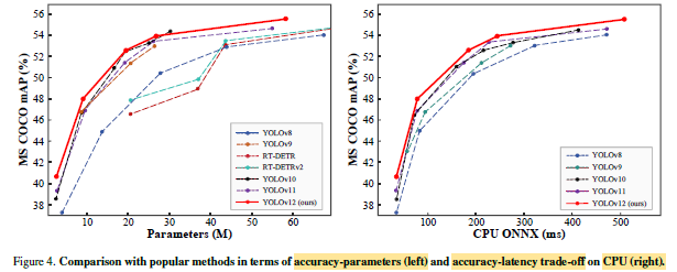
YOLOv12 surpasses other competitors with a more advantageous boundary, highlighting its efficiency across diverse hardware platforms.
2.2. Visualization
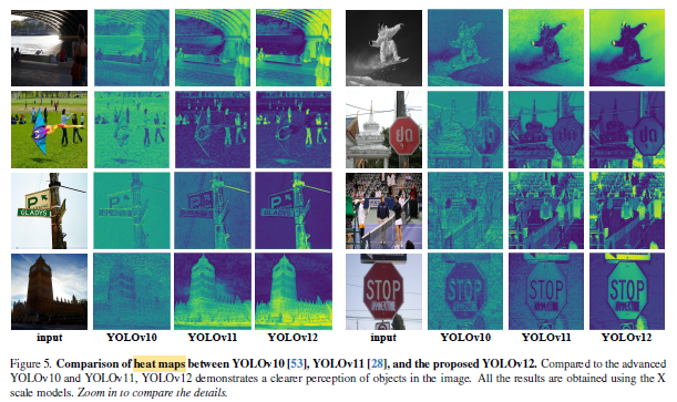
YOLOv12 produces clearer object contours and more precise foreground activation, indicating improved perception.
- (There are also ablation studies for all proposed components. Please feel free to read the papers if interested.)
