Recurrent Seq2Seq Autoencoder on HSS Corpus

Sik-Ho Tsang

·

Follow

4 min read

·

Jun 15, 2024

--

Listen

Share

Deep Unsupervised Representation Learning for Abnormal Heart Sound Classification
Seq2Seq Autoencoder on HSS, by University of Augsburg, Technische Universität München, Imperial College London, and Shenzhen University General Hospital
2018 EMBC, Over 30 Citations (Sik-Ho Tsang @ Medium)

Phonocardiogram (PCG)/Heart Sound Classification
2013 … 2023 … [CTENN] [Bispectrum + ViT] 2024 [MWRS-BFSC + CNN2D]
==== My Other Paper Readings Are Also Over Here ====

• The suitability of deep feature representations as learnt by sequence to sequence Autoencoders is explored on HSS corpus.

Outline

1. Recurrent Sequence to Sequence (Seq2Seq) Autoencoders
2. ComParE Acoustic Feature Set and Bag-of-Audio-Words (BoAW) Baselines
3. Results

1. Recurrent Sequence to Sequence (Seq2Seq) Autoencoders

1.1. Flowchart

• (a): First, Mel-spectrograms are obtained from the raw heartbeat recordings.
• (b): A sequence to sequence (Seq2Seq) Autoencoder is then trained on these extracted spectra that are considered as time-dependent sequences of frequency vectors.
• (c): After Autoencoder training, the learnt representations of the Mel-spectrograms are then generated for use as feature vectors for the corresponding instances.
• (d): Finally, a classifier is trained on the feature sets to predict the labels of the heartbeat recordings.

1.2. Mel-spectrogram Extraction

• First, the power spectra of heartbeat recordings is generated using periodic Hann windows with variable width w and overlap 0.5w.
• Subsequently, a given number Nmel of log-scaled Mel frequency bands are computed from the spectra.
• The Mel-spectra values are normalised in [-1, 1].
• Authors also study whether removing some background noise from the spectrograms improves system performance. This is achieved by clipping amplitudes below a certain threshold .

1.3. Recurrent Sequence to Sequence (Seq2Seq) Autoencoders

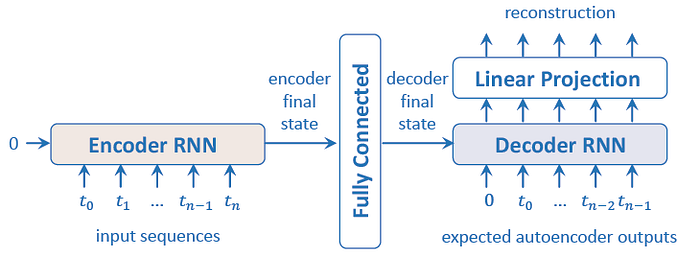
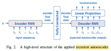
• Each sequence represent the amplitudes of the Nmel Mel frequency bands within one audio segment and is then fed to a multilayered encoder RNN. The hidden state of the encoder is then updated regarding to the input frequency vector. Accordingly, the final hidden state of the encoder RNN comprises information regarding the full input sequence.
• This final hidden state is reconstructed applying a fully connected layer.
• Another multilayered decoder RNN is used to rebuild the original input sequence from the reconstructed feature.
• Particularly, a unidirectional encoder RNN and a bidirectional decoder RNN are used.
• The encoder RNN has Nlayer=2 layers and each layer contains Nunit =256 Gated Recurrent Units (GRUs).
• Root mean square error (RMSE) is used as loss function.
• Dropout of 0.2 is applied to the outputs of each recurrent layer.
• Moreover, gradients with absolute value above 2 are clipped.

2. ComParE Acoustic Feature Set and Bag-of-Audio-Words (BoAW) Baselines

2.1. ComParE Acoustic Feature Set

• This feature set comprises a range of prosodic, spectral, cepstral, and voice quality low-level descriptor (LLD) — prosodic, spectral, cepstral, and voice quality — contours, to which statistical functionals such as the mean, standard deviation, percentiles and quartiles, linear regression descriptors, and local minima/maxima related descriptors are applied to produce a 6373 dimensional static feature vector.

2.2. Bag-of-Audio-Words (BoAW)

• BoAW involves the quantisation of acoustic LLDs to form a sparse fixed length histogram (bag) representation of an audio clip.
• All BoAW representations were generated from the 65 LLDs and corresponding deltas in the COMPARE feature set.
• Prior to quantisation, the LLDs were normalised to zero mean and unit variance.
• Codebook sizes of 250, 500, 1000 are considered.

2.3. SVM

• A linear SVM classifier is used for the above features.

3. Results

3.1. HSS Dataset

• As outlined, the corpus has been divided into three classes: (i) normal, (ii) mild, and (iii) moderate/severe.
• These classes are divided into participant-independent training, development, and test sets with 502, 180, and 163 audio instances, respectively.
• The gender and age classes are evenly distributed. In summary, there are 100 normal, 35 mild, and 35 moderate/severe subjects.

3.2. Performance Comparison

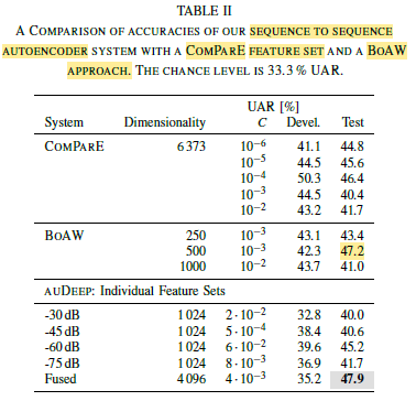
• The strongest development set UAR, 50.3% (cf. Table II), was achieved using a system based on the COMPARE feature set and a SVM. However, this system had a noticeable drop in performance on the HSS test partition indicating possible overfitting.
• For the conventional (non-deep) approaches, the strongest test set partition UAR, 47.2% (cf. Table II) was achieved using a BoAW approach with a codebook size of 500, and a SVM.
• For the deep recurrent approach, four feature sets are extracted by amplitude clipping below thresholds of -30dB, -45dB, -60dB, and -75dB. These learnt representations achieved a weaker performance than the conventional feature sets on the development partition. This could be due to the small amount of data for training.
• Moreover, an early fusion of the four learnt deep feature vectors obtain the highest UAR, 47.9% (cf. Table II) on the test set.