[Paper] DeepBIQ: Deep Learning for Blind IQA (Image Quality Assessment)

Using CaffeNet, Outperforms IQA-CNN & IQA-CNN++

Examples from the LIVE In the Wild IQ Chall. DB

In this story, On the use of deep learning for blind image quality assessment (DeepBIQ), by University of Milano-Bicocca, is presented. I read this because I recently study IQA/VQA. In this paper:

• Features of subregions are extracted by fine-tuned convolutional neural networks (CNNs) as a generic image description, then input to SVR to regress the image quality scores.
• The image quality is estimated by average-pooling the scores predicted on multiple subregions of the original image.
• This proposed approach is named DeepBIQ.

This is a paper in 2017 Springer JSVIP (Signal, Image and Video Processing). (Sik-Ho Tsang @ Medium)

Outline

1. CaffeNet: Network Architecture
2. Pretrained CNN
3. Pooling Strategies
4. Experimental Results

1. CaffeNet: Network Architecture

CaffeNet: Network Architecture

• CaffeNet, i.e. AlexNet without the use of group convolution, is used for feature extraction. The length of the feature vector is 4096 as shown above.
• (If interested, please feel free to read CaffeNet.)
• Then, a support vector regression (SVR) machine with a linear kernel is exploited to learn a mapping function from the CNN features to the perceived quality scores (i.e., MOS).

2. Pretrained CNN

• Three pretrained network is considered.

1. ImageNet-CNN: CNN trained on trained on 1.2 million images of ImageNet (ILSVRC 2012).
2. Places-CNN: CNN trained on 2.5 million images of the Places Database for scene recognition.
3. ImageNet+Places-CNN: Trained using 3.5 million images from 1183 categories.
4. Fine-tuned CNN: Fine-tuning the network by substituting the last fully connected layer of a pre-trained CNN with a new one initialized with random values. The new layer is trained from scratch. In this case, The CNN is discriminatively fine-tuned to classify image subregions into five MOS classes.

3. Pooling Strategies

• CNN features are computed on multiple subregions (i.e., crops) of the input image.
• Each crop covers almost 21% of the original image (227×227 out of 500×500 pixels). Thus, the use of multiple crops permits to evaluate the local quality.
• The final image quality is then computed by pooling the evaluation of each single crop.
• Three pooling strategies are considered.

1. Feature pooling information fusion is performed element by element on the subregion feature vectors to generate a single feature vector using a minimum, average, or maximum pooling operators.
2. Feature concatenation information fusion is performed by concatenating the subregion feature vectors in a single longer feature vector.
3. Prediction pooling information fusion is performed on the predicted quality scores. The SVR predicts a quality score for each image crop, and these scores are then fused using a minimum, average, or maximum pooling operators.

4. Experimental Results

• The LIVE In the Wild IQ Challenge DB is used. It contains 1162 images with resolution equal to 500×500 pixels affected by diverse authentic distortions and genuine artifacts such as low-light noise and blur, motion-induced blur, over and underexposure, compression errors.

4.1. Pretrained CNN (Exp. I)

Performance of Pretrained CNN

• ImageNet+Places-CNN obtains the best performance as it is trained with much more images.

4.2. Feature and Prediction Pooling (Exp. II)

Performance of Feature and Prediction Pooling

• ImageNet+Places-CNN is used.
• The first scheme is feature pooling that can be seen as an early fusion approach, performing element-wise fusion on the feature vectors.
• The second scheme is feature concatenation, performing information fusion by concatenating the multiple feature vectors into a single feature vector.
• The third scheme is prediction pooling that can be seen as a late fusion approach, where information fusion is performed on the predicted quality scores.
• The results obtained by feature average-pooling are statistically better.

4.3. Fine-tuned CNN (Exp. III)

Performance of Fine-tuned CNN

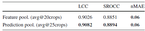
• The results obtained by prediction average-pooling are statistically better than those obtained by feature average-pooling.
• The test time requires about 20 ms for CNN.

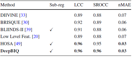
4.4. SOTA Comparison

Median LCC, SROCC, and nMAE across 10 train–test random splits of the LIVE In the Wild IQ Chall. DB

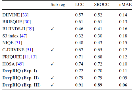
• We can see that the use of a pre-trained CNN on the whole image is able to give slightly better results than the best in the state of the art.
• The use of multiple crops with average-pooled features is able to improve LCC and SROCC with respect to the best method in the state of the art by 0.08 and 0.11, respectively.
• Finally, the use of the fine-tuned CNN with multiple image crops and average-pooled predictions is able to improve LCC and SROCC by 0.20 and 0.21 respectively.

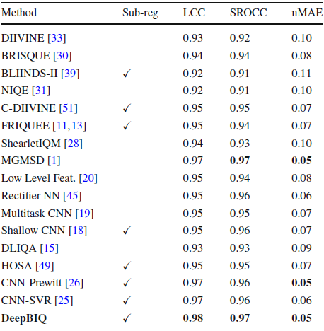
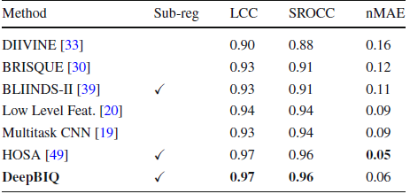
4.5. Other Datasets

Median LCC, SROCC, and nMAE across 100 random splits of the legacy LIVE Image Quality Assessment DB

Median LCC, SROCC, and nMAE across 100 random splits of the CSIQ

Median LCC, SROCC, and nMAE across 100 random splits of the TID2008

Median LCC, SROCC, and nMAE across 100 random splits of the TID2013

• From the above results, it is possible to see that DeepBIQ is able to obtain the best performance in terms of LCC, SROCC, and nMAE.
• It outperforms such as IQA-CNN (Shallow CNN) & IQA-CNN++ (Multitask CNN).

Reference

[2017 JSVIP] [DeepBIQ]
On the use of deep learning for blind image quality assessment

Image Quality Assessment (IQA)

FR: [DeepSim] [DeepIQA]
NR: [IQA-CNN] [IQA-CNN++] [DeepCNN] [DeepIQA] [DeepBIQ] [MEON]

My Other Previous Reviews