[Paper] NetAdapt: Platform-Aware Neural Network Adaptation for Mobile Applications (Image Classification)

Outperforms MorphNet, MobileNetV2 & MobileNetV1.

NetAdapt

In this story, NetAdapt: Platform-Aware Neural Network Adaptation for Mobile Applications (NetAdapt), by Massachusetts Institute of Technology (MIT), and Google Inc., is presented. In this paper:

• By using NetAdapt. the pre-trained network is simplified progressively until the resource budget is met while maximizing the accuracy.

This is a paper in 2018 ECCV with over 190 citations. (Sik-Ho Tsang @ Medium)

Outline

1. Problem Formulation
2. NetAdapt
3. Ablation Study
4. Experimental Results

1. Problem Formulation

• NetAdapt aims to solve the following:

• where Net is a simplified network, Acc(·) computes the accuracy, Resj(·) evaluates the direct metric for resource consumption of the j-th resource, and Budj is the budget of the jth resource.
• The resource can be latency, energy, or memory.
• NetAdapt focuses on latency.
• NetAdapt breaks this problem into the following series of easier problems and solves it iteratively:

• where Neti is the network generated by the ith iteration, and Net0 is the initial pretrained network.
• The constraints (i.e., current resource budget Resj(Neti−1)−ΔRi,j) gradually become tighter as for more iterations.
• This is referred to as “resource reduction schedule”, which is similar to the concept of learning rate schedule.

2. NetAdapt

2.1. Overall Flow

Algorithm flow of NetAdapt

• Each iteration solves the 2nd equation in Section 1 by reducing the number of filters in a single CONV or FC layer (the Choose # of Filters and Choose Which Filters blocks in the above figure).
• The number of filters to remove from a layer is guided by empirical measurements. And NetAdapt will remove entire filters.
• The simplified network is then fine-tuned for a short length of time in order to restore some accuracy (the Short-Term Fine-Tune block).
• In each iteration, the above three steps (highlighted in bold) are applied.
• As a result, NetAdapt generates K (i.e., the number of CONV and FC layers) network proposals in one iteration, each of which has a single layer modified from the previous iteration.
• The network proposal with the highest accuracy is carried over to the next iteration (the Pick Highest Accuracy block).
• Finally, once the target budget is met, the chosen network is fine-tuned again until convergence (the Long-Term Fine-Tune block).

2.2. Details for Each Step

• Choose Number of Filters: This step focuses on determining how many filters to preserve in a specific layer based on empirical measurements.
• The change in the resource consumption of other layers needs to be factored in.
• Choose Which Filters: This step chooses which filters to preserve based on the architecture from the previous step.
• The magnitude-based method is used to keep the algorithm simple. In this work, the N filters that have the largest ℓ2-norm magnitude will be kept.
• Short-/Long-Term Fine-Tune: Both involve network-wise end-to-end fine-tuning. Short-term fine-tune has fewer iterations than long-term fine-tune.
• Short-term Fine-Tune is to regain the accuracy after simplifying the network. It is especially important while adapting small networks with a large resource reduction because otherwise the accuracy will drop to zero.
• Once the final adapted network is obtained, long-Term Fine-Tune is performed.

2.3. Latency Estimation

layer-wise look-up tables

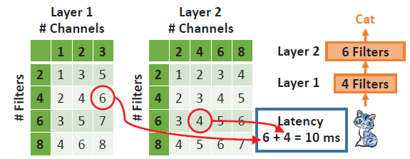
• We can look up the table of each layer, and sum up the layer-wise measurements to estimate the network-wise resource consumption.

The comparison between the estimated latency (using layer-wise look-up tables) and the real latency

• Layers with the same shape and feature map size only need to be measured once.
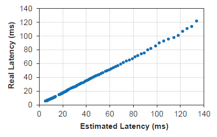
• The estimated latency (the sum of layer-wise latency from the layer-wise look-up tables) and the real latency on a single large core of Google Pixel 1 CPU are highly correlated, as shown above.

3. Ablation Study

3.1. Impact of Direct Metrics

The comparison between NetAdapt and other benchmarks

• NetAdapt outperforms the benchmark algorithms with lower numbers of MACs and higher accuracy.
• The network with lower numbers of MACs may not necessarily be faster. This shows the necessity of incorporating direct measurements into the optimization flow.

3.2. Impact of Short-Term Fine-Tuning

The accuracy of different short-term fine-tuning iterations

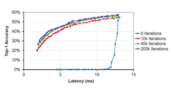
• The accuracy rapidly drops to nearly zero if no short-term fine-tuning is performed.
• After fine-tuning a network for a short amount of time (ten thousand iterations), the accuracy is always kept above 20%.
• Using forty thousand iterations leads to a good accuracy versus speed trade-off for the small MobileNetV1.

3.3. Impact of Long-Term Fine-Tuning

The comparison between before and after long-term fine-tuning (LFT)

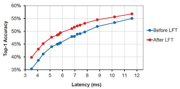
• Although the short-term fine-tuning preserves the accuracy well, the long-term fine-tuning can still increase the accuracy by up to another 4.5% or 3.4% on average.

3.4. Impact of Resource Reduction Schedules

The influence of resource reduction schedules

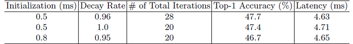
• Empirically, using a larger resource reduction at each iteration increases the adaptation speed (i.e., reducing the total number of adaptation iterations) at the cost of accuracy.
• The result suggests that a smaller initial resource reduction with a slower decay is preferable.

3.5. Analysis of Adapted Network Architecture

NetAdapt and the multipliers generate different simplified networks

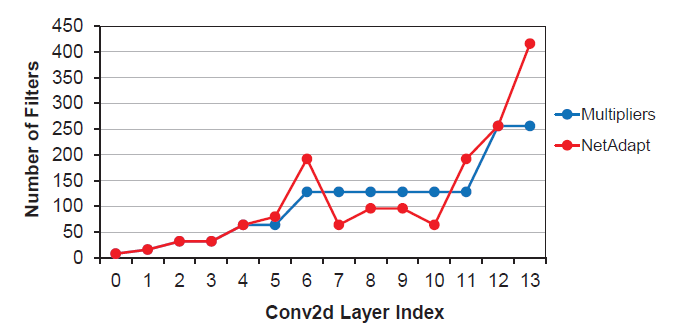
• Multipliers: It is a width multiplier method to reduce the feature maps.
• NetAdapt removes more filters in layers 7 to 10, but fewer in layer 6. It is hypothesized that when the feature map resolution is reduced, more filters are needed to avoid creating an information bottleneck.
• NetAdapt keeps more filters in layer 13. One possible explanation is that the ImageNet dataset contains one thousand classes, so more feature maps are needed by the last FC layer to do the correct classification.

4. Experimental Results

• Multipliers: Width multiplier scales the number of filters by a percentage across all convolutional (CONV) and fully-connected (FC) layers,
• MorphNet: Reducing feature maps using sparsifying regularization.
• ADC: Simplification algorithm based on reinforcement learning.
• Ten thousand images are preserved from the training set, ten images per class, as the holdout set.
• The new training set without the holdout images is used to perform short-term fine-tuning, and the holdout set is used to pick the highest accuracy network out of the simplified networks at each iteration.
• The whole training set is used for the long-term fine-tuning.
• Mobile CPU: Google’s TensorFlow Lite engine
• Mobile GPU: Qualcomm’s Snapdragon Neural Processing Engine (SNPE)

4.1. Adapting Small MobileNetV1 on a Mobile CPU

Performance of Small MobileNetV1 for mobile CPU of Google Pixel 1

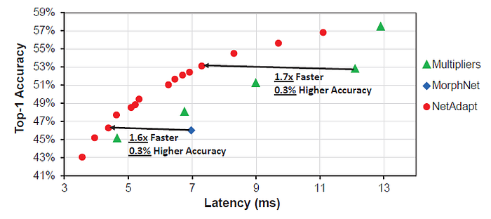
• NetAdapt outperforms the multipliers by up to 1.7× faster with the same or higher accuracy.
• For MorphNet, NetAdapt’s result is 1.6× faster with 0.3% higher accuracy.

4.2. Adapting Large MobileNetV1 on a Mobile CPU

Performance of Large MobileNetV1 for mobile CPU of Google Pixel 1

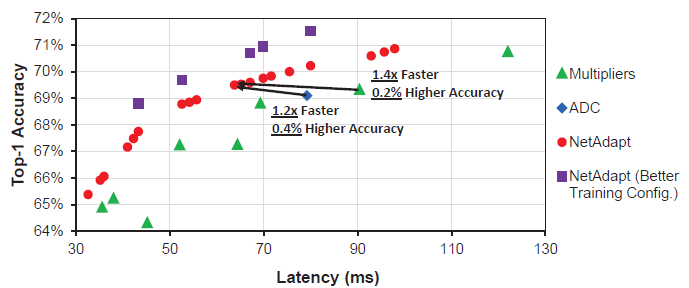
• NetAdapt achieves higher accuracy than the multipliers and ADC while increasing the speed by 1.4× and 1.2×, respectively.
• After simply adding dropout and label smoothing, the accuracy can be increased by 1.3%.

4.3. Adapting Large MobileNetV1 on a Mobile GPU

Performance of Large MobileNetV1 for mobile GPU of Samsung Galaxy S8

• NetAdapt outperforms other benchmark algorithms by up to 1.2× speed-up with higher accuracy.
• When the better training configuration is applied as previously described, the accuracy can be further increased by 1.3%.

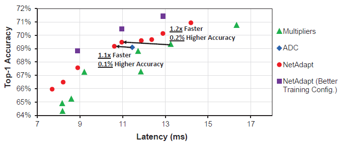
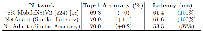
4.4. Adapting Large MobileNetV2 on a Mobile CPU

Performance of Large MobileNetV2 on a mobile CPU of Google Pixel 1

• Authors only adapt individual inner (expansion) layers or reduce all bottleneck layers of the same resolution in lockstep.
• NetAdapt achieves 1.1% higher accuracy or 1.2× faster speed than the multipliers.

Reference

[2018 ECCV] [NetAdapt]
NetAdapt: Platform-Aware Neural Network Adaptation for Mobile Applications

Image Classification

1989-1998: [LeNet]
2012–2014: [AlexNet & CaffeNet] [Maxout] [NIN] [ZFNet] [SPPNet]
2015: [VGGNet] [Highway] [PReLU-Net] [STN] [DeepImage] [GoogLeNet / Inception-v1] [BN-Inception / Inception-v2]
2016: [SqueezeNet] [Inception-v3] [ResNet] [Pre-Activation ResNet] [RiR] [Stochastic Depth] [WRN] [Trimps-Soushen]
2017: [Inception-v4] [Xception] [MobileNetV1] [Shake-Shake] [Cutout] [FractalNet] [PolyNet] [ResNeXt] [DenseNet] [PyramidNet] [DRN] [DPN] [Residual Attention Network] [IGCNet / IGCV1] [Deep Roots]
2018: [RoR] [DMRNet / DFN-MR] [MSDNet] [ShuffleNet V1] [SENet] [NASNet] [MobileNetV2] [CondenseNet] [IGCV2] [IGCV3] [FishNet] [SqueezeNext] [ENAS] [PNASNet] [ShuffleNet V2] [BAM] [CBAM] [MorphNet] [NetAdapt]
2019: [ResNet-38] [AmoebaNet] [ESPNetv2] [MnasNet] [Single-Path NAS] [DARTS] [ProxylessNAS]

My Other Previous Paper Readings