Review — Multi-task Self-Supervised Visual Learning

Pretrain Using Multiple Pretext Tasks to Improve Downstream Task Accuracy

Multi-task Self-Supervised Visual Learning
Doersch ICCV’17, by DeepMind, and VGG, University of Oxford
2017 ICCV, Over 400 Citations (Sik-Ho Tsang @ Medium)
Self-Supervised Learning, Representation Learning, Image Classification, Object Detection, Depth Prediction

• In this paper, 4 different self-supervised tasks using ResNet-101 are combined to jointly train a network.
• Lasso regularization is used to factorize the information in its representation, and methods for “harmonizing” network inputs in order to learn a more unified representation.

Outline

1. Multi-Task Network
2. Model Fine-Tuning
3. Experimental Results

1. Multi-Task Network

The structure of our multi-task network based on ResNet-101, with block 3 having 23 residual units. a) Naïve shared-trunk approach, where each “head” is attached to the output of block 3. b) the lasso architecture, where each “head” receives a linear combination of unit outputs within block3, weighted by the matrix , which is trained to be sparse.

• Three architectures are described:

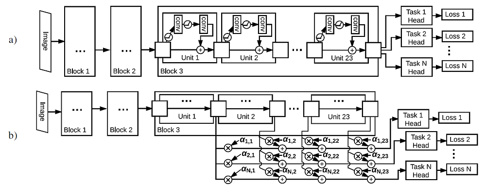
1. First, the (naïve) multi-task network that has a common trunk and a head for each task (figure a)
2. Second, the lasso extension of this architecture (figure b) that enables the training to determine the combination of layers to use for each self-supervised task; and,
3. Third, a method for harmonizing input channels across self-supervision tasks.

1.1. Common Trunk

• ResNet-101, as in Pre-Activation ResNet, is used. The entire architecture up to the end of block 3 are kept.
• This same block3 representation is used to solve all tasks and evaluations (see figure a). Thus, the “trunk” has an output with 1024 channels, and consists of 88 convolution layers with roughly 30 million parameters.

Each task has a separate loss, and has extra layers in a “head,” which may have a complicated structure.

• For instance, the relative position (Context Prediction) and Exemplar tasks have a Siamese architecture. This is achieved by passing all patches through the trunk as a single batch, and then rearranging the elements in the batch to make pairs (or triplets) of representations to be processed by the head.
• At each training iteration, only one of the heads is active. However, gradients are averaged across many iterations where different heads are active, meaning that the overall loss is a sum of the losses of different tasks.

4 Self-supervised tasks are used: Relative Position (Context Prediction), Colorization, Exemplar, and Motion Segmentation (Motion Masks).

1.2. Separating Features via Lasso

• Different tasks require different features. If the features are factorized into different tasks, then the network can select from the discovered feature groups while training on the evaluation tasks.
• A linear combination of skip layers is passed to each head. Concretely, each task has a set of coefficients, one for each of the 23 candidate layers in block 3. The representation that’s fed into each task head is a sum of the layer activations weighted by these task-specific coefficients.
• A lasso (L1) penalty is proposed to encourage the combination to be sparse, which therefore encourages the network to concentrate all of the information required by a single task into a small number of layers.
• Thus, when fine-tuning on a new task, these task-specific layers can be quickly selected or rejected as a group.
• The representation passed to the head for task n is then:

• where N is the number of self-supervised tasks, M is the number of residual units in block 3, and Unitm is the output of residual unit m.
• To ensure sparsity, an L1 penalty is added on the entries of α to the objective function. A similar α matrix is created for the set of evaluation tasks.

1.3. Harmonizing Network Inputs

• Each self-supervised task pre-processes its data differently.
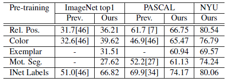
• To “harmonize,” relative position (Context Prediction)’s preprocessing is replaced with the same preprocessing used for Colorization: images are converted to Lab, and the a and b channels are discarded (The L channel is replicated by 3 times).

1.4. Distributed Network Training

Distributed training setup

• Each machine trains the network on a single task.
• Several GPU machines are allocated for each task, and gradients from each task are synchronized and aggregated with separate RMSProp optimizers.
• A hybrid approach is used that gradients are accumulated from all workers that are working on a single task, and then have the parameter servers apply the aggregated gradients from a single task when ready, without synchronizing with other tasks.
• Experiments found that this approach resulted in faster learning than either purely synchronous or purely asynchronous training, and in particular, was more stable than asynchronous training.
• 64 GPUs are used in parallel, and checkpoints are saved every roughly 2.4K GPU (NVIDIA K40) hours.

2. Model Fine-Tuning

2.1. ImageNet

• After self-supervised training, a single linear classification layer (a softmax) to the network at the end of block 3, and train on the full ImageNet training set.
• All pre-trained weights are frozen during training.

2.2. PASCAL VOC 2007 Detection

• Fast R-CNN is used, which trains a single network base with multiple heads for object proposals, box classification, and box localization.
• All network weights are fine-tuned.

2.3. NYU V2 Depth Prediction

• ResNet-50 is used. The block 3 outputs are directly fed into the up-projection layers.
• All network weights are fine-tuned.

2. Experimental Results

2.1. Individual Self-Supervised Training Performance

Individual Self-Supervised Training Performance

• Of the self-supervised pre-training methods, relative position (Context Prediction) and Colorization are the top performers, with relative position (Context Prediction) winning on PASCAL and NYU, and Colorization winning on ImageNet-frozen.
• Remarkably, relative position (Context Prediction) performs on-par with ImageNet pre-training on depth prediction, and the gap is just 7.5% mAP on PASCAL.
• The only task where the gap remains large is the ImageNet evaluation itself, which is not surprising since the ImageNet pretraining and evaluation use the same labels.
• Motion segmentation (Motion Masks) and Exemplar training are somewhat worse than the others, with Exemplar worst on Pascal and NYU, and motion segmentation (Motion Masks) worst on ImageNet.

Comparison of performance for different self-supervised methods over time

• After 16.8K GPU hours, performance is plateauing but has not completely saturated.
• Interestingly, on the ImageNet frozen evaluation, where Colorization is winning, the gap relative to relative position (Context Prediction) is growing.
• Also, while most algorithms slowly improve performance with training time, Exemplar training doesn’t fit this pattern.

2.2. Naïve Multi-Task Combination of Self-Supervision Tasks

Comparison of various combinations of self-supervised tasks RP: Relative Position (Context Prediction); Col: Colorization; Ex: Exemplar Nets; MS: Motion Segmentation (Motion Masks). Metrics: ImageNet: Recall@5; PASCAL: mAP; NYU: % Pixels below 1.25.

• Adding either Colorization or Exemplar leads to more than 6 points gain on ImageNet.
• Adding both Colorization and Exemplar gives a further 2% boost.
• The best-performing method was a combination of all four self-supervised tasks.

2.3. Harmonization

Comparison of methods with and without harmonization, H: harmonization

• There are large improvements on ImageNet.
• The other two evaluation tasks do not show any improvement with harmonization.
• This suggests that our networks are actually quite good at dealing with stark differences between pre-training data domains when the features are fine-tuned at test time.

2.4. Lasso

Comparison of performance with and without the lasso technique for factorizing representations, for a network trained on all four self-supervised tasks for 16.8K GPU-hours.

• There are four cases: no lasso, lasso only on the evaluation tasks, lasso only at pre-training time, and lasso in both self-supervised training and evaluation.

• The gap between ImageNet pre-trained and self-supervision pre-trained with four tasks is nearly closed for the VOC detection evaluation, and completely closed for NYU depth.

Reference

[2017 ICCV] [Doersch ICCV’17]
Multi-task Self-Supervised Visual Learning

Self-Supervised Learning

2008–2010 [Stacked Denoising Autoencoders] 2014 [Exemplar-CNN] 2015 [Context Prediction] [Wang ICCV’15] 2016 [Context Encoders] [Colorization] [Jigsaw Puzzles] 2017 [L³-Net] [Split-Brain Auto] [Mean Teacher] [Motion Masks] [Doersch ICCV’17] 2018 [RotNet/Image Rotations] [DeepCluster] [CPC/CPCv1]

My Other Previous Paper Readings