Review — Π-Model, Temporal Ensembling: Temporal Ensembling for Semi-Supervised Learning

Stochastic Augmentation, Network Dropout, & Momentum Encoder are Used

Π-Model & Temporal Ensembling

Temporal Ensembling for Semi-Supervised Learning
Π-Model, Temporal Ensembling, by NVIDIA
2017 ICLR, Over 1400 Citations (Sik-Ho Tsang @ Medium)
Semi-Supervised Learning, Image Classification

• Predictions are under different regularization and input augmentation conditions.
• Self-ensembling is used, which is similar to momentum encoder in MoCo.

Outline

1. Π-Model
2. Temporal Ensembling
3. Experimental Results

1. Π-Model

Π-Model

Π-Model

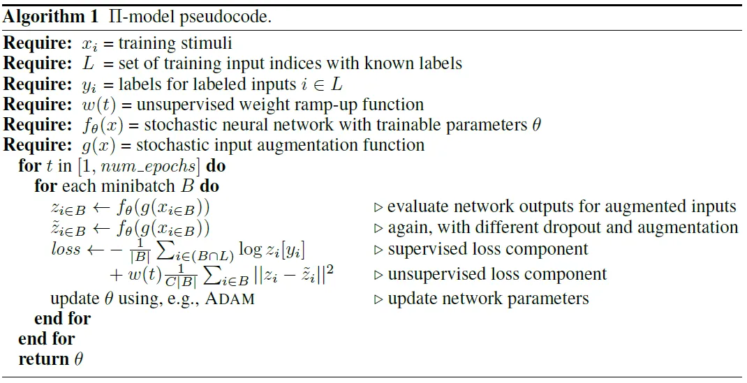
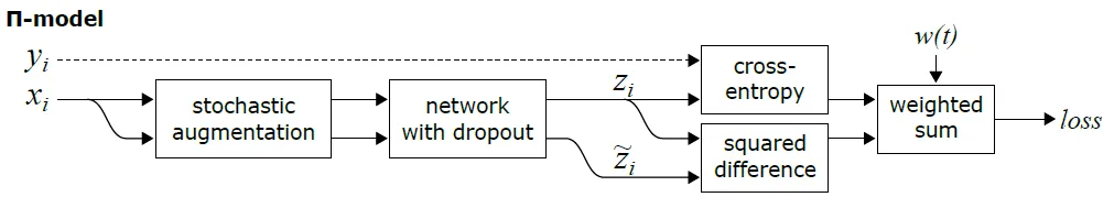
• During training, the network evaluates each training input xi twice, resulting in prediction vectors zi and ~zi.
• Loss function consists of two components:

1. The first component is the standard cross-entropy loss, evaluated for labeled inputs only.
2. The second component, evaluated for all inputs, penalizes different predictions for the same training input xi by taking the mean square difference between the prediction vectors zi and ~zi.

• Because of Dropout regularization, as well as Gaussian noise and augmentations, there is difference between the prediction vectors zi and ~zi given the same original input xi. However, the labels should be the same since they are coming from the same original input xi. Thus, minimizing the MSE between zi and ~zi is reasonable.
• To combine the supervised and unsupervised loss terms, a time-dependent weighting function w(t) is used to scale/balance the two terms, where t is the epoch number. This w(t) ramps up, starting from zero, along a Gaussian curve during the first 80 training epochs.
• Compared to Γ-Model, instead of having one “clean” and one “corrupted” branch as in Γ-Model, augmentation and noise are applied to the inputs for both branches.
• (The two-branch architecture for zi and ~zi is commonly used in later self-supervised learning.)

2. Temporal Ensembling

Temporal Ensembling

Temporal Ensembling

• The main difference to the Π-model is that the network and augmentations are evaluated only once per input per epoch.
• And the target vectors ~z for the unsupervised loss component are based on prior network evaluations instead of a second evaluation of the network:

• where α is a momentum term.
• Because of Dropout regularization and stochastic augmentation, Z thus contains a weighted average of the outputs of an ensemble of networks f from previous training epochs, with recent epochs having larger weight than distant epochs.
• (This is the idea used by later self-supervised learning such as MoCo.)
• For generating the training targets ~z, the startup bias in Z needs to be corrected by dividing by factor (1-α^t). Since on the first training epoch, Z and ~z are zero as no data from previous epochs is available. For this reason, the unsupervised weight ramp-up function w(t) is also zero on the first training epoch.
• The benefits of temporal ensembling compared to Π-model are twofold:

1. First, the training is faster because the network is evaluated only once per input on each epoch.
2. Second, the training targets ~z can be expected to be less noisy than with Π-model.

3. Experimental Results

3.1. Network Architecture

Network Architecture

• A network architecture similar to VGGNet is used.

3.2. CIFAR-10

CIFAR-10 results with 4000 labels, averages of 10 runs (4 runs for all labels)

• Π-model obtains 16.55% error rate on CIFAR-10.
• Enabling the standard set of augmentations further reduces the error rate by 4.2 percentage points to 12.36%.
• Temporal ensembling is slightly better still at 12.16%, while being twice as fast to train.

3.3. SVHN

SVHN results for 500 and 1000 labels, averages of 10 runs (4 runs for all labels)

• With the most commonly used 1000 labels, an improvement of 2.7 percentage points is observed, from 8.11% (Sajjadi NIPS’16) to 5.43% without augmentation, and further to 4.42% with standard augmentations.
• When augmentations were enabled, temporal ensembling further reduced the error rate to 5.12%. In this test the difference between Π-model and temporal ensembling was quite significant at 1.5 percentage points.

3.4. CIFAR-100

CIFAR-100 results with 10000 labels, averages of 10 runs (4 runs for all labels)

• With 10000 labeled images, Π-model obtains error rates of 43.43% and 38.65% without and with augmentation, respectively. These correspond to 7.8 and 5.9 percentage point improvements compared to supervised learning with labeled inputs only.

3.5. CIFAR-100 + Tiny Images

CIFAR-100 + Tiny Images results, averages of 10 runs

• Unlabeled extra data from Tiny Images dataset, is used. One with randomly selected 500k extra images, most not corresponding to any of the CIFAR-100 categories, and another with a restricted set of 237k images from the categories that correspond to those found in the CIFAR-100 dataset.
• Unlabeled extra images improved the error rate by 2.7 percentage points (from 26.30% to 23.63%).
• However, restricting the extra data to categories that are present in CIFAR-100 did not improve the classification accuracy further.

Reference

[2017 ICLR] [Π-Model, Temporal Ensembling]
Temporal Ensembling for Semi-Supervised Learning

Pretraining or Weakly/Semi-Supervised Learning

2013 [Pseudo-Label (PL)] 2015 [Ladder Network, Γ-Model] 2016 [Sajjadi NIPS’16] 2017 [Mean Teacher] [PATE & PATE-G] [Π-Model, Temporal Ensembling] 2018 [WSL] 2019 [Billion-Scale] [Label Propagation] [Rethinking ImageNet Pre-training] 2020 [BiT] [Noisy Student] [SimCLRv2]

My Other Previous Paper Readings