Review — CMC: Contrastive Multiview Coding

Representation Learning Using Multiview Data

Inputs Come From Different Views, Learn the View-Invariant Feature Representations

Contrastive Multiview Coding
CMC, by MIT CSAIL, and Google Research
2020 ECCV, Over 800 Citations (

Sik-Ho Tsang

@ Medium)
Contrastive Learning, Multiview Learning, Unsupervised Learning, Self-Supervised Learning, Image Classification, Video Classification, Action Recognition

• There is a classic hypothesis saying that a powerful representation is one that models view-invariant factors.
• A representation is learnt that aims to maximize mutual information between different views of the same scene but is otherwise compact.

Outline

1. Predictive Learning vs Contrastive Learning
2. Contrastive Learning with Two Views
3. Contrastive Learning with More than Two Views
4. Experimental Results

1. Predictive Learning vs Contrastive Learning

Predictive Coding vs Contrastive Learning

• Consider a collection of M views of the data, denoted as V1, …, VM. For each view Vi, we denote vi as a random variable representing samples following vi~P(Vi).
• (a) Predictive coding for two views: Cross-view prediction (Top) learns latent representations that predict one view from another, with loss measured in the output space:
• (b) Contrastive learning: Representations are learnt by contrasting congruent and incongruent views, with loss measured in representation space.
• This paper focuses on contrastive learning.

2. Contrastive Learning with Two Views

Contrastive learning from two views: the luminance channel (L) of an image and the ab-color channel

2.1. Contrastive Loss

• Given a dataset of V1 and V2 that consists of a collection of samples {vi1, vi2} where i is from 1 to N samples.
• Contrasting congruent and incongruent pairs, i.e. samples from the joint distribution x~p(v1, v2) or x={vi1, vi2}, which called positives, versus samples from the product of marginals, y~p(v1)p(v2) or y = {vi1, vj2}, which called negatives.
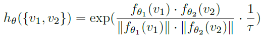
• hθ(.) is trained to achieve a high value for positive pairs and low for negative pairs.
• Based on NCE concept such as the one in Instance Discrimination, the function is trained to correctly select a single positive sample x out of a set S={x, y1, y2, …, yk} that contains k negative samples:

• To construct S, simply fix one view and enumerate positives and negatives from the other view, allowing to rewrite the objective:

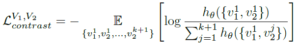
• where k is the number of negative samples vj2 for a given sample v11.

In practice, k can be extremely large (e.g., 1.2 million in ImageNet). Two approximations are used for tractable computation.

2.2. Contrastive Learning Implementation

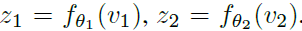
• Two encoders fθ1() and fθ2() with parameters θ1 and θ2 respectively, are to be learnt to extract the latent representations z1 and z2 from two views v1 and v2 respectively:

• Their cosine similarity is computed as score and adjust its dynamic range by a hyper-parameter τ:

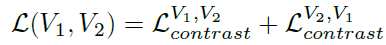
• We can treat view V1 as anchor and enumerates over V2, and also treat view V2 as anchor and enumerates over V1. Thus the two-view loss is:

• After the contrastive learning phase, the representation z1, z2, or the concatenation of both, [z1, z2], can be used for further actions.

2.3. Memory Bank

• Following Instance Discrimination, a memory bank is maintained to store latent features for each training sample.
• Therefore, using memory bank can efficiently retrieve m negative samples from the memory buffer to pair with each positive sample without recomputing their features.
• The memory bank is dynamically updated with features computed on the fly.

2.4. Connecting to Mutual Information (Proofs in Appendix of the Paper)

• The optimal critic hθ* is proportional to the density ratio between the joint distribution p(z1, z2) and the product of marginals p(z1)p(z2):

• It is proved that minimizing the objective L actually maximizes the lower bound on the mutual information I(zi, zj):

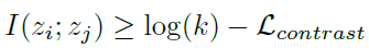
• where k is the number of negative pairs in sample set S. The dependency on k also suggests that using more negative samples can lead to an improved representation.

3. Contrastive Learning with More than Two Views

Graphical models and information diagrams [1] associated with the core view and full graph paradigms, for the case of 4 views, which gives a total of 6 learning objectives.

• Suppose there is a collection of M views V1, …, VM.
• The number in each partition of the diagram indicates how many of the pairwise objectives, L(Vi, Vj), that partition contributes to.

3.1. (a) Core View

• The “core view” formulation sets apart one view that we want to optimize over, say V1, and builds pair-wise representations between V1 and each other view Vj, j>1, by optimizing the sum of a set of pair-wise objectives:

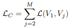
• As in the figure, the mutual information between V2 and V3 or V2 and V4 is completely ignored in the core view paradigm.

3.2. (b) Full Graph

• More general formulation is the “full graph” where we consider all pairs (i, j), i≠ j, and build (n 2) relationships in all:

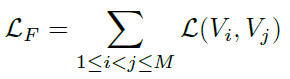
• As in the figure, full graph formulation captures more information between different views.
• Another benefit of the full graph formulation is that it can handle missing information (e.g. missing views) in a natural manner.

4. Experimental Results

4.1. ImageNet

Views: {L, ab}

• Given a dataset of RGB images, we convert them to the Lab image color space, and split each image into L and ab channels.
• Two color spaces are tried, {L, ab} and {Y, DbDr}.
• During contrastive learning, L and ab from the same image are treated as the positive pair, and ab channels from other randomly selected images are treated as a negative pair.
• Encoders are deep network such as AlexNet and ResNet. Representations can be obtained from intermediate layers. By concatenating representations layer-wise from these two encoders, the final representation of an input image is obtained.
• The quality of such a representation is evaluated by freezing the weights of encoder and training linear classifier on top of each layer.
• τ=0.07 and 16384 negatives are used.

Top-1 / Top-5 Single crop classification accuracy (%) on ImageNet with a supervised logistic regression classifier.

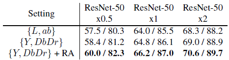
• {L, ab} achieves 68.3% top-1 single crop accuracy with ResNet50×2 for each view, and switching to {Y, DbDr} further brings about 0.7% improvement.
• On top of it, strengthening data augmentation with RandAugment (RA)[14] yields better or comparable results to other state-of-the-art methods.

4.2. Video Classification / Action Recognition

Views: {it, ft, it+k}

• Given images it at time t and it+k at time t+k, optical flow ft is extracted using TV-L1 algorithm from two modalities. Thus, 3 views are obtained.
• The negative sample can be a random frame from another randomly chosen video, or the flow corresponding to a random frame in another randomly chosen video.
• Two CaffeNets are trained on UCF101, for extracting features from images and optical flows, respectively.
• The action recognition CaffeNet up to conv5 is initialized using the weights from the pre-trained RGB CaffeNet.

Test accuracy (%) on UCF-101 which evaluates task transferability and on HMDB-51 which evaluates task and dataset transferability.

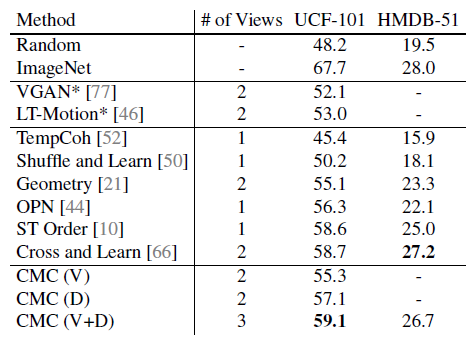
Increasing the number of views of the data from 2 to 3 (using both streams instead of one) provides a boost for UCF-101.

4.3. Extending CMC to More Views (NYU RGBD)

Views: {L, ab, Depth, Segmentation}

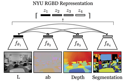
• On NYU RGB-D dataset, consider the task of predicting semantic labels from the representation of L, the 2–4 view cases contrast L with ab, and then sequentially add depth and surface normals.
• The views are (in order of inclusion): L, ab, depth and surface normals.
• U-Net is used to perform the segmentation task.

Intersection over Union (IoU) (left) and Pixel Accuracy (right) for the NYU-Depth-V2 dataset, against number of views

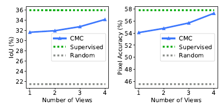
The performance steadily improves as new views are added.

Results on the task of predicting semantic labels from L channel representation which is learnt using the patch-based contrastive loss and all 4 views.

• Supervised learning provides the upper bound.

CMC produces high quality feature maps even though it’s unaware of the downstream task.

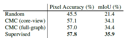
4.4. Is CMC Improving All Views?

Performance on the task of using single view v to predict the semantic labels, where v can be L, ab, depth or surface normal.

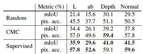
The performance of the representations learned by CMC using full-graph significantly outperforms that of randomly projected representations, and approaches the performance of the fully supervised representations.

4.5. Predictive Learning vs. Contrastive Learning

Compare predictive learning with contrastive learning by evaluating the learned encoder on unseen dataset and task.

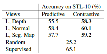
• Three sets of view pairs on the NYU-Depth dataset are considered: (1) L and depth, (2) L and surface normals, and (3) L and segmentation map.
• For each of them, two identical encoders are trained for L, one using contrastive learning and the other with predictive learning.
• Then the representation quality is evaluated by training a linear classifier on top of these encoders on the STL-10 dataset.

Contrastive learning consistently outperforms predictive learning in this scenario where both the task and the dataset are unknown.

• Though only 1.3K images are used the unsupervised stage, from a dataset much different from the target dataset STL-10, the object recognition accuracy is close to the supervised method.

4.6. How Does Mutual Information Affect Representation Quality?

(Left) Classification accuracy against estimated MI between channels of different color spaces; (Right) Classification accuracy vs estimated MI between patches at different distances (distance in pixels is denoted next to each data point). MI estimated using MINE

• Cross-view representation learning is effective because it results in a kind of information minimization, discarding nuisance factors that are not shared between the views.

CMC wants to maximize the “good” information — the signal — in the representations, while minimizing the “bad” information — the noise.

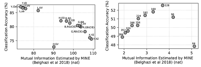
• Two hypothesis are tested: learning representations on images with different color spaces forming the two views; and learning representations on pairs of patches extracted from an image, separated by varying spatial distance.
• Left: The plots clearly show that using color spaces with minimal mutual information give the best downstream accuracy.
• Right: Views with too little or too much MI perform worse; a sweet spot in the middle exists which gives the best representation.

If two views share no information, then, in principle, there is no incentive for CMC to learn anything. If two views share all their information, no nuisances are discarded.

References

[2020 ECCV] [CMC]
Contrastive Multiview Coding

CMC

Unsupervised/Self-Supervised Learning

2008–2010 [Stacked Denoising Autoencoders] 2014 [Exemplar-CNN] 2015 [Context Prediction] [Wang ICCV’15] 2016 [Context Encoders] [Colorization] [Jigsaw Puzzles] 2017 [L³-Net] [Split-Brain Auto] [Motion Masks] [Doersch ICCV’17] 2018 [RotNet/Image Rotations] [DeepCluster] [CPC/CPCv1] [Instance Discrimination] 2020 [CMC]

My Other Previous Paper Readings