Review — AS-MLP: An Axial Shifted MLP Architecture for Vision
Pure MLP With Axial Shift, Comparable With Swin Transformer
AS-MLP: An Axial Shifted MLP Architecture for Vision
AS-MLP, by ShanghaiTech University, Tencent, Shanghai Engineering Research Center of Intelligent Vision and Imaging & Shanghai Engineering Research Center of Energy Efficient and Custom AI IC
2022 ICLR, Over 40 Citations (Sik-Ho Tsang @ Medium)
Image Classification, MLP
- Pure MLP architecture is designed, with the design of the receptive field size and dilation of blocks.
- It is the first work to apply MLP-based architecture to object detection.
Outline
- Axial Shifted MLP (AS-MLP)
- AS-MLP Block
- Complexity & Sampling Location Comparisons
- Experimental Results
1. Axial Shifted MLP (AS-MLP)

1.1. Overall Architecture for AS-MLP-T
- Given an RGB image I, AS-MLP performs the patch partition operation to multiple patch tokens with the patch size of 4×4, the combination of all tokens has the size of 48×H/4×W/4.
- AS-MLP has four stages in total and there are different numbers of AS-MLP blocks in different stages. The final output feature will be used for image classification.
- In Stage 1, a linear embedding and the AS-MLP blocks are adopted for each token. The output has the dimension of C×H/4×W/4, where C is the number of channels.
- Stage 2 first performs patch merging on the features outputted from the previous stage, which groups the neighbor 2×2 patches to obtain a feature with the size of 4C×H/8×W/8 and then a linear layer is adopted to warp the feature size to 2C×H/8×W/8, followed by the cascaded AS-MLP blocks.
- Stage 3 and Stage 4 have similar structures to Stage 2.
2.5. AS-MLP Variants
- There are AS-MLP-Tiny (AS-MLP-T), AS-MLP-Small (AS-MLP-S), AS-MLP-Base (AS-MLP-B), and AS-MLP (mobile) respectively.
- AS-MLP-T: C=96, the number of blocks in 4 stages = {2, 2, 6, 2}.
- AS-MLP-S: C=96, the number of blocks in 4 stages = {2, 2, 18, 2}.
- AS-MLP-B: C=128, the number of blocks in 4 stages = {2, 2, 18, 2}.
- AS-MLP (mobile): C=64, the number of blocks in 4 stages = {2, 2, 2, 2}.
2. AS-MLP Block

2.1. AS-MLP Block Structure
- It mainly consists of the Norm layer, Axial Shift operation, MLP, and residual connection.
- In the Axial Shift operation, the channel projection, vertical shift, and horizontal shift are utilized to extract features, where the channel projection maps the feature with a linear layer.
Vertical shift and horizontal shift are responsible for the feature translation along the spatial directions.
2.2. Axial-Shift Example
- The input has the dimension of C×h×w. For convenience, h is omitted and C=3, w=5 are used in the figure (b).
- When the shift size is 3, the input feature is split into three parts and they are shifted by {-1, 0, 1} units along the horizontal direction, respectively.
- Zero padding is performed in the gray area.
- After that, the features in the dashed box will be taken out and used for the next channel projection.
In the process of both shifts, since the feature performs different shift units, the information from different spatial positions can be combined together.
In the next channel projection operation, information from different spatial locations can fully flow and interact.
3. Complexity & Sampling Location Comparisons
3.1. Complexity Comparisons
- In the Transformer-based architecture, the multi-head self-attention (MSA) is usually adopted.
- In Swin Transformer, Window MSA (W-MSA) is used, with window size of M.
- In AS-MLP, there is only Axially Shift (AS) the feature from the previous layer, which does not require any multiplication and addition operations.
- The time cost of Axial Shift is very low and almost irrelevant to the shift size.
- Each Axial shift operation in Figure (a) only has four channel projection operations, which has the computation complexity 4hwC².
- The complexities of MSA, W-MSA and AS are as follows:
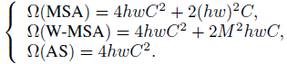
- Therefore, the AS-MLP architecture has slightly less complexity than Swin Transformer.
3.2. Sampling Locations
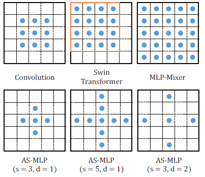
- Unlike MLP-Mixer, AS-MLP pays more attention to the local dependencies through axial shift of features and channel projection.
4. Experimental Results
4.1. ImageNet

AS-MLP outperforms other MLP-based architectures when keeping similar parameters and FLOPs.
- e.g., AS-MLP-S obtains higher top-1 accuracy (83.1%) with fewer parameters than Mixer-B/16 (76.4%) and ViP-Medium/7 (82.7%).
Furthermore, it achieves competitive performance compared with Transformer-based architectures.
- e.g., AS-MLP-B (83.3%) vs. Swin-B (83.3%).
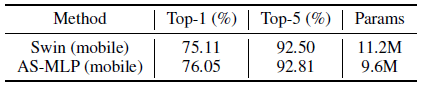
AS-MLP (mobile) significantly exceeds Swin Transformer in the mobile setting (76.05% vs. 75.11%).
4.2. Ablation Studies
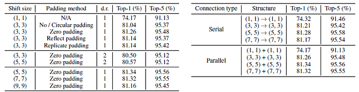
- All ablations are conducted based on the AS-MLP-T.
- (Left) Different Configurations: Three findings as follows:
- ‘Zero padding’ is more suitable for the design of AS-MLP block than other padding methods.
- Increasing the dilation rate slightly reduces the performance of AS-MLP, which is consistent with CNN-based architecture. Dilation is usually used for semantic segmentation rather than image classification.
- When expanding the shift size, the accuracy will increase first and then decrease. When shift size is 9, the network pays too much attention to the global dependencies, thus neglecting the extraction of local features, which leads to lower accuracy.
Therefore, the configuration (shift size = 5, zero padding, dilation rate = 1) in all experiments are used, including object detection and semantic segmentation.
- (Right) Connection Type: Parallel connection consistently outperforms serial connection in terms of different shift sizes.
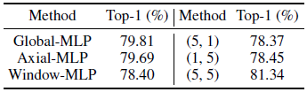
- Here five baselines are designed: i) Global-MLP; ii) Axial-MLP; iii) Window-MLP; iv) shift size (5, 1); v) shift size (1, 5).
- The first three baselines are designed from the perspective of how to use MLP for feature fusion at different positions, and the latter two are designed from the perspective of the axial shift in a single direction.
AS-MLP block with shift size (5, 5) outperforms other baselines.
4.3. Object Detection & Instance Segmentation
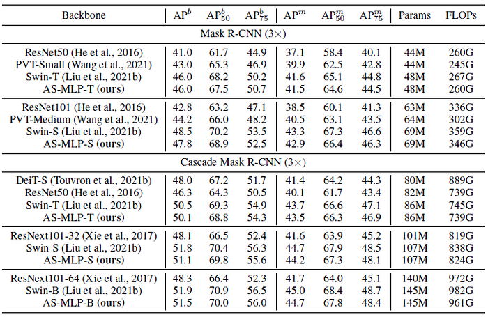
AS-MLP achieves comparable performance with Swin Transformer in the similar resource limitation.
- To be specific, Cascade Mask R-CNN + Swin-B achieves 51.9 APb with 145M parameters and 982 GFLOPs, and Cascade Mask R-CNN + AS-MLP-B obtains 51.5 APb with 145M parameters and 961 GFLOPs.

4.4. Semantic Segmentation
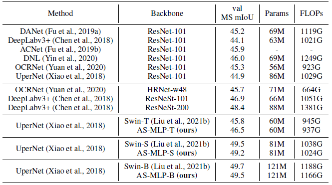
- With slightly lower FLOPs, AS-MLP-T achieves better result than Swin-T (46.5 vs. 45.8 MS mIoU).
- For the large model, UPerNet + Swin-B has 49.7 MS mIoU with 121M parameters and 1188 GFLOPs, and UPerNet + AS-MLP-B has 49.5 MS mIoU with 121M parameters and 1166 GFLOPs.
This shows the effectiveness of AS-MLP architecture in processing the downstream task.
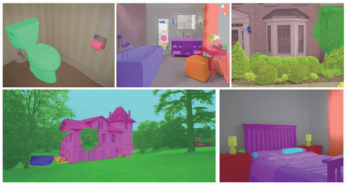
4.5. Attended Areas
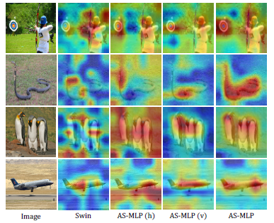
- The first column shows the image from ImageNet, and the second column shows the activation heatmap of the last layer of Swin Transformer (Swin-B).
- The third, fourth, and fifth columns respectively indicate the response after the horizontal shift (AS-MLP (h)), the vertical shift (AS-MLP (v)) and the combination of both in the last layer of AS-MLP (AS-MLP-B).
AS-MLP can better focus on object regions compared to Swin Transformer.
By axially shifting channels of the feature map, AS-MLP is able to obtain the information flow from different axial directions, which captures the local dependencies.
Reference
[2022 ICLR] [AS-MLP]
AS-MLP: An Axial Shifted MLP Architecture for Vision
1.1. Image Classification
1989 … 2022 [ConvNeXt] [PVTv2] [ViT-G] [AS-MLP]