Review — ConvNeXt: A ConvNet for the 2020s
ConvNeXt, ConvNet Without Any Self-Attention, Outperforms Swin Transformer

A ConvNet for the 2020s
ConvNeXt, by Facebook AI Research (FAIR), and UC Berkeley
2022 CVPR, Over 80 Citations (Sik-Ho Tsang @ Medium)
Image Classification, Convolutional Neural Network, CNN, ResNet, Vision Transformer, Swin Transformer
- Vision Transformers have been dominant in 2021. Hierarchical Transformers (e.g., Swin Transformers) that reintroduced several ConvNet priors.
- In this paper, authors gradually “modernize” a standard ResNet toward the design of a Vision Transformer, and discover several key components, e.g.: Training Techniques, Macro Design, ResNeXt-ify, Inverted Bottleneck, Large Kernel, and Micro Design.
- Finally, a network family, ConvNeXt, is formed.
Outline
- Training Techniques
- Macro Design
- ResNeXt-ify
- Inverted Bottleneck
- Large Kernel Size
- Micro Design
- ConvNeXt
- Experimental Results
1. Training Techniques

- Starting Point: ResNet-50 is the model used as a starting point.
- Baseline: Similar training techniques used to train Vision Transformers are to train the original ResNet-50 to obtain much improved results.
The training recipe is close to DeiT’s and Swin Transformer’s.
- The training is extended to 300 epochs. AdamW optimizer is used.
- Data augmentation techniques such as mixup, CutMix, RandAugment, Random Erasing, and regularization schemes including Stochastic Depth and Label Smoothing in Inception-v3, are used. (Details in Paper Appendix A.1.)
This enhanced training recipe increased the performance of the ResNet-50 model from 76.1% to 78.8% (+2.7%), implying that a significant portion of the performance difference between traditional ConvNets and Vision Transformers may be due to the training techniques.
2. Macro Design

- There are two interesting design considerations: the stage compute ratio, and the “stem cell” structure.
2.1. Changing Stage Compute Ratio
- ResNet: The original design of the computation distribution across stages in ResNet was largely empirical. The heavy “res4” stage was meant to be compatible with downstream tasks like object detection, where a detector head operates on the 14×14 feature plane.
- Transformer: Swin-T, on the other hand, followed the same principle but with a slightly different stage compute ratio of 1:1:3:1. For larger Swin Transformers, the ratio is 1:1:9:1.
Following the design, authors adjust the number of blocks in each stage from (3, 4, 6, 3) in ResNet-50 to (3, 3, 9, 3), which also aligns the FLOPs with Swin-T. This improves the model accuracy from 78.8% to 79.4%.
2.2. Changing Stem to “Patchify”
- ResNet: The stem cell in standard ResNet contains a 7×7 convolution layer with stride 2, followed by a max pool, which results in a 4 downsampling of the input images.
- Transformer: In Vision Transformers, a more aggressive “patchify” strategy is used as the stem cell, which corresponds to a large kernel size (e.g. kernel size = 14 or 16) and non-overlapping convolution. Swin Transformer uses a similar “patchify” layer, but with a smaller patch size of 4 to accommodate the architecture’s multi-stage design.
The ResNet-style stem cell is replaced with a patchify layer implemented using a 4×4, stride 4 convolutional layer. The accuracy has changed from 79.4% to 79.5%.
This suggests that the stem cell in a ResNet may be substituted with a simpler “patchify” layer as in ViT which will result in similar performance. The “patchify stem” (4×4 non-overlapping convolution) is used in the network.
3. ResNeXt-ify

- ResNeXt: At a high level, ResNeXt’s guiding principle is to “use more groups, expand width”. ResNeXt employs grouped convolution for the 3×3 conv layer in a bottleneck block.
- MobileNet or Xception: Here, depthwise convolution (as used in MobileNet or Xception), a special case of grouped convolution where the number of groups equals the number of channels, is used. Depthwise convolution is similar to the weighted sum operation in self-attention. The combination of depthwise conv and 1×1 convs leads to a separation of spatial and channel mixing, a property shared by Vision Transformers.
Following the strategy proposed in ResNeXt, the network width is increased to the same number of channels as Swin-T’s (from 64 to 96). This brings the network performance to 80.5% with increased FLOPs (5.3G).
4. Inverted Bottleneck


- Transformer: One important design in every Transformer block is that it creates an inverted bottleneck, i.e., the hidden dimension of the MLP block is four times wider than the input dimension.
From (a) to (b): The inverted bottleneck design is explored. Despite the increased FLOPs for the depthwise convolution layer, this change reduces the whole network FLOPs to 4.6G. Interestingly, this results in slightly improved performance (80.5% to 80.6%).
5. Large Kernel Size


- ConvNet: Such as VGGNet, it stacks small kernel-sized (3×3) conv layers.
- Transformer: Although Swin Transformers reintroduced the local window to the self-attention block, the window size is at least 7×7, significantly larger than the ResNe(X)t kernel size of 3×3.
5.1. Moving Up Depthwise Conv Layer.
From (b) to (c): To explore large kernels, the proposed prerequisite is to move up the position of the depthwise conv layer. That is a design decision also evident in Transformers: the MSA block is placed prior to the MLP layers. This intermediate step reduces the FLOPs to 4.1G, resulting in a temporary performance degradation to 79.9%.
5.2. Increasing the Kernel Size
By experimenting with several kernel sizes, including 3, 5, 7, 9, and 11. The network’s performance increases from 79.9% (3×3) to 80.6% (7×7). 7×7 depthwise conv is used in each block.
6. Micro Design


6.1. Replacing ReLU with GELU
- GELU, which can be thought of as a smoother variant of ReLU, is utilized in the most advanced Transformers, including Google’s BERT and OpenAI’s GPT-2, and, most recently, ViTs.
ReLU can be substituted with GELU, although the accuracy stays unchanged (80.6%).
6.2. Fewer Activation Functions
- Transformer: There is only one activation function present in the MLP block.
All GELU layers are eliminated from the residual block except for one between two 1×1 layers, replicating the style of a Transformer block. This process improves the result by 0.7% to 81.3%, practically matching the performance of Swin-T. Thus only a single GELU activation is used in each block.
6.3. Fewer Normalization Layers
- Transformer blocks usually have fewer normalization layers as well.
Here, two BatchNorm (BN) layers are removed, leaving only one BN layer before the conv 1×1 layers. This further boosts the performance to 81.4%, already surpassing Swin-T’s result.
6.4. Substituting BN with LN
The proposed ConvNet model does not have any difficulties training with LN; in fact, the performance is slightly better, obtaining an accuracy of 81.5%. From now on, one LayerNorm is used as the choice of normalization in each residual block.
6.5. Separate Downsampling Layers
- ResNet: the spatial downsampling is achieved by the residual block at the start of each stage, using 3×3 conv with stride 2 (and 1×1 conv with stride 2 at the shortcut connection).
- Swin Transformers: a separate downsampling layer is added between stages.
A similar strategy is explored in which 2×2 conv layers with stride 2 are used for spatial downsampling. This modification surprisingly leads to diverged training. One LN before each downsampling layer, one LN after the stem, and one LN after the final global average pooling, are added, to stabilize the training. The accuracy is increased to 82.0%, significantly exceeding Swin-T’s 81.3%.
7. ConvNeXt
7.1. All Improvements Together

- The above figure summarizes all the above improvements, which finally surpasses the Swin Transformer.
- These designs are not novel but they have all been researched separately, but not collectively, over the last decade.
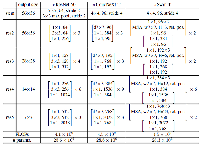
7.2. Detailed Architecture
7.3. ConvNeXt Variants

- Different ConvNeXt variants, ConvNeXt-T/S/B/L, are designed to be of similar complexities to Swin-T/S/B/L. ConvNeXt-T/B is the end product of the “modernizing” procedure on ResNet-50/200 regime, respectively.
- In addition, a larger ConvNeXt-XL is built to further test the scalability of ConvNeXt. The variants only differ in the number of channels C, and the number of blocks B in each stage. Following both ResNets and Swin Transformers, the number of channels doubles at each new stage.
8. Experimental Results
8.1. ImageNet

8.1.1. ImageNet-1K (Upper Part of Table)
- ConvNeXt competes favorably with two strong ConvNet baselines (RegNet and EfficientNet) in terms of the accuracy-computation trade-off, as well as the inference throughputs.
- ConvNeXt also outperforms Swin Transformer of similar complexities across the board, sometimes with a substantial margin (e.g. 0.8% for ConvNeXt-T). ConvNeXts also enjoy improved throughput compared to Swin Transformers.
- e.g.: A highlight from the results is ConvNeXt-B at 384²: it outperforms Swin-B by 0.6% (85.1% vs. 84.5%), but with 12.5% higher inference throughput (95.7 vs. 85.1 image/s).
- An improved result of 85.5% is obtained when further scaling to ConvNeXt-L.
8.1.2. Pretraining Using ImageNet-22K on ImageNet-1K (Lower Part of Table)
- ConvNeXts still perform on par or better than similarly-sized Swin Transformers, with slightly higher throughput.
- Additionally, ConvNeXt-XL model achieves an accuracy of 87.8% — a decent improvement over ConvNeXt-L at 384², demonstrating that ConvNeXts are scalable architectures.
- ConvNeXt is able to outperform EfficientNetV2, further demonstrating the importance of large-scale training.
8.2. Isotropic ConvNeXt vs. ViT
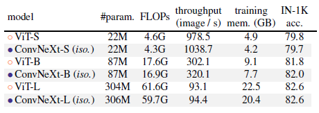
- This part is to examine if ConvNeXt block design is generalizable to ViT-style isotropic architectures which have no downsampling layers and keep the same feature resolutions (e.g. 14×14) at all depths.
ConvNeXt can perform generally on par with ViT, showing that ConvNeXt block design is competitive when used in non-hierarchical models.
8.3. Object Detection and Segmentation on COCO

- Mask R-CNN and Cascade R-CNN are fine-tuned on the COCO dataset with ConvNeXt backbones. Multi-scale training, AdamW optimizer, and a 3× schedule, are used.
- Training Cascade R-CNN using ConvNeXt-B backbone consumes 17.4GB of peak memory with a per-GPU batch size of 2, while the reference number for Swin-B is 18.5GB.
Across different model complexities, ConvNeXt achieves on-par or better performance than Swin Transformer.
- When scaled up to bigger models (ConvNeXt-B/L/XL) pre-trained on ImageNet-22K, in many cases ConvNeXt is significantly better (e.g. +1.0 AP) than Swin Transformers in terms of box and mask AP.
8.4. Semantic Segmentation on ADE20K
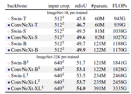
ConvNeXt models can achieve competitive performance across different model capacities, further validating the effectiveness of architecture design.
(While Transformers in computer vision are the mainstream research in 2021, ConvNeXt outperforms Swin Transformer now, which is awesome!)
Reference
[2022 CVPR] [ConvNeXt]
A ConvNet for the 2020s
Image Classification
2021: [Learned Resizer] [Vision Transformer, ViT] [ResNet Strikes Back] [DeiT] [EfficientNetV2] [MLP-Mixer] [T2T-ViT] [Swin Transformer] [CaiT] [ResMLP] [ResNet-RS] [NFNet] [PVT, PVTv1] [CvT] [HaloNet] [TNT] [CoAtNet] [Focal Transformer] [TResNet] 2022: [ConvNeXt]
