Review — MLP-Mixer: An all-MLP Architecture for Vision

Network Composes of Only MLPs, No CNN, No Transformer

MLP-Mixer: An all-MLP Architecture for Vision
MLP-Mixer, by Google Research, Brain Team
2021 NeurIPS, Over 190 Citations (Sik-Ho Tsang @ Medium)
Image Classification, Multi-Layer Perceptron, MLP

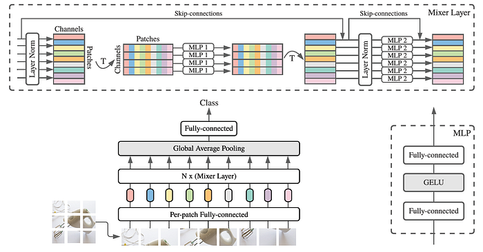
• MLP-Mixer contains two types of layers: one with MLPs applied independently to image patches (i.e. “mixing” the per-location features), and one with MLPs applied across patches (i.e. “mixing” spatial information).
• MLP-Mixer attains competitive scores on image classification benchmarks despite its simplicity.

Outline

1. MLP-Mixer: Network Architecture
2. Experimental Results

1. MLP-Mixer: Network Architecture

MLP-Mixer: Network Architecture

• The network design is most similar to Transformers.
• Mixer takes as input a sequence of S non-overlapping image patches, each one projected to a desired hidden dimension C. This results in a two-dimensional real-valued input table, X with the size of S×C.
• If the original input image has resolution (H, W), and each patch has resolution (P, P), then the number of patches is S=HW/P². All patches are linearly projected with the same projection matrix.
• Mixer consists of multiple layers of identical size, and each layer consists of two MLP blocks.
• The first one is the token-mixing MLP: it acts on columns of X (i.e. it is applied to a transposed input table XΤ), maps from size of S to size of S, and is shared across all columns.
• The second one is the channel-mixing MLP: it acts on rows of X, maps from size of C to size of C, and is shared across all rows.
• Each MLP block contains two fully-connected layers and a GELU nonlinearity GELU applied independently to each row of its input data tensor.
• Mixer layers can be written as follows:

• where σ is GELU.
• DS and DC, dimensions of S and C respectively, are tunable hidden widths in the token-mixing and channel-mixing MLPs, respectively. DS is selected independently of the number of input patches. Therefore, the computational complexity of the network is linear in the number of input patches, unlike ViT whose complexity is quadratic.
• Also, as mentioned, the same MLP is applied to every row/column of X, this parameter tying prevents the architecture from growing too fast when increasing the hidden dimension C or the sequence length S and leads to significant memory savings.
• Aside from the MLP layers, Mixer uses other standard architectural components: skip-connections and layer normalization.
• Unlike ViTs, Mixer does not use position embeddings.
• Finally, Mixer uses a standard classification head with the global average pooling layer followed by a linear classifier.

Specifications of the Mixer architectures. “B”, “L”, and “H” stand for base, large, and huge, “B/16” means the model of base scale with patches of resolution 16×16

• The Mixer is scaled into B, L, and H model sizes.

2. Experimental Results

2.1. Main Results

Transfer performance, inference throughput, and training cost.

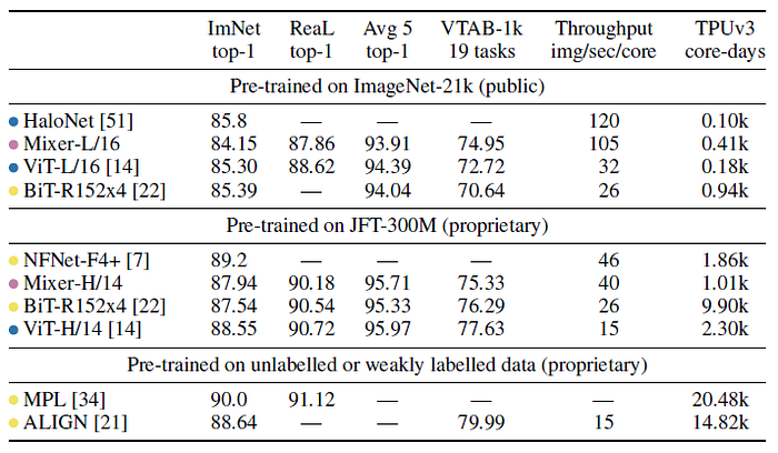
• The MLP-based Mixer models are marked with pink, convolution-based models with yellow, and attention-based models with blue. HaloNets use both attention and convolutions and is marked with blue.
• When pre-trained on ImageNet-21k with additional regularization, Mixer achieves an overall strong performance (84.15% top-1 on ImageNet), although slightly inferior to other models.
• When the size of the upstream dataset increases, Mixer’s performance improves significantly. In particular, Mixer-H/14 achieves 87.94% top-1 accuracy on ImageNet, which is 0.5% better than BiT-ResNet152×4 and only 0.5% lower than ViT-H/14.
• Remarkably, Mixer-H/14 runs 2.5 times faster than ViT-H/14 and almost twice as fast as BiT.

Left: ImageNet accuracy/training cost Pareto frontier (dashed line), Right: Mixer (solid) catches or exceeds BiT (dotted) and ViT (dashed) as the data size grows

• Left: In terms of the accuracy-compute trade-off, Mixer is competitive with more conventional neural network architectures. The figure also demonstrates a clear correlation between the total pre-training cost and the downstream accuracy.
• Right: Every point on a curve uses the same pre-training compute; they correspond to pre-training on 3%, 10%, 30%, and 100% of JFT-300M for 233, 70, 23, and 7 epochs, respectively. Additional points at ~3B correspond to pre-training on an even larger JFT-3B dataset for the same number of total steps.

Mixer improves more rapidly with data than ResNets, or even ViT. The gap between large Mixer and ViT models shrinks.

2.2. The Role of Model Scale

ImageNet validation top-1 accuracy vs. total pre-training compute (left) and throughput (right) (All models are pre-trained on JFT-300M and fine-tuned at resolution 224.)

Performance of Mixer and other models from the literature across various model and pre-training dataset scales

• Compared with BiT: When pre-trained on the smallest subset of JFT-300M, all Mixer models strongly overfit. BiT models also overfit, but to a lesser extent, possibly due to the strong inductive biases associated with the convolutions. As the dataset increases, the performance of both Mixer-L/32 and Mixer-L/16 grows faster than BiT; Mixer-L/16 keeps improving, while the BiT model plateaus.
• Compared with ViT: The performance gap between Mixer-L/16 and ViT-L/16 shrinks with data scale. It appears that Mixer benefits from the growing dataset size even more than ViT.

Also, Mixer is more invariant to input permutations such as pixel shuffling, please feel free to read the paper if interested.

1 story for each day, consecutive 30-story challenge accomplished. :)

Reference

[2021 NeurIPS] [MLP-Mixer]
MLP-Mixer: An all-MLP Architecture for Vision

Image Classification

1989–2019 … 2020: [Random Erasing (RE)] [SAOL] [AdderNet] [FixEfficientNet] [BiT] [RandAugment] [ImageNet-ReaL]
2021: [Learned Resizer] [Vision Transformer, ViT] [ResNet Strikes Back] [DeiT] [EfficientNetV2] [MLP-Mixer]

My Other Previous Paper Readings