Review — Learning Deep Transformer Models for Machine Translation
Pre-Norm Transformer, Layer Normalization First
Learning Deep Transformer Models for Machine Translation
Pre-Norm Transformer, by Northeastern University, NiuTrans Co., Ltd., Kingsoft AI Lab, and University of Macau
2019 ACL, Over 200 Citations (Sik-Ho Tsang @ Medium)
Natural Language Processing, NLP, Machine Translation, Transformer
- Two novel techniques are proposed:
- A proper use of layer normalization is proposed, called pre-norm Transformer, and;
- A novel way of passing the combination of previous layers to the next.
Outline
- Pre-Norm Transformer
- Dynamic Linear Combination of Layers (DLCL)
- Experimental Results
1. Pre-Norm Transformer

1.1. Original Post-Norm Transformer
- On the encoder side, there are a number of identical stacked layers. Each of them is composed of a self-attention sub-layer and a feed-forward sub-layer.
- The attention model used in Transformer is multi-head attention, and its output is fed into a fully connected feed-forward network.
- For Transformer, it is not easy to train stacked layers, residual connections and layer normalization are adopted:

- where xl and xl+1 are the input and output of the l-th sub-layer, and yl is the intermediate output followed by the post-processing function f().
- Layer normalization is adopted to reduce the variance of sub-layer output, and it is placed after the element-wise residual addition:

- It can be seen as a post-processing step of the output.
1.2. Proposed Pre-Norm Transformer
- In contrast, layer normalization is applied to the input of every sub-layer:

- The above equation regards layer normalization as a part of the sub-layer, and does nothing for post-processing of the residual connection.
1.3. Gradients of Post-Norm
- A stack of L sub-layers are used as an example. Let E be the loss used to measure how many errors occur in system prediction, and xL be the output of the topmost sub-layer.
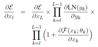
- For post-norm Transformer, given a sub-layer l, the differential of E with respect to xl can be computed by the chain rule, and we have:

The above equation is inefficient for passing gradients back because the residual connection is not a bypass of the layer normalization unit.
1.4. Gradients of Pre-Norm
- Likewise, we have the gradient for pre-norm:

Obviously, the above equation for pre-norm establishes a direct way to pass error gradient ∂E/∂xL from top to bottom. Its merit lies in that the number of product items on the right side does not depend on the depth of the stack.
2. Dynamic Linear Combination of Layers (DLCL)

DLCL is proposed to make direct links with all previous layers and offers efficient access to lower-level representations in a deep stack.
- Let {y0, …, yl} be the output of layers 0~l. The input of layer l+1 is defined to be:

- where G() is a linear function that merges previously generated values {y0, …, yl} into a new value.
- For pre-norm Transformer, G() is defined as:

where W(l+1)k is a learnable scalar and weights each incoming layer in a linear manner. The above equation provides a way to learn preference of layers in different levels of the stack.
- For post-norm, G() can be redefined as:

3. Experimental Results
3.1. SOTA Comparison

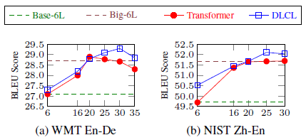
- When increasing the encoder depth, e.g. L=20, the vanilla Transformer failed to train. On the contrary, post-norm DLCL solves this issue and achieves the best result when L=25.
Pre-norm slightly underperforms the post-norm counterpart in shallow networks, pre-norm Transformer benefits more from the increase in encoder depth.
- Pre-norm is easier to optimize than post-norm in deep networks. Beyond that, a 30-layer encoder is successfully trained, resulting in a further improvement of 0.4 BLEU points. This is 0.6 BLEU points higher than the pre-norm Transformer-Big.
Although the best score of 29.3 is the same as Ott et al. (2018), the proposed approach only requires 3.5× fewer training epochs than theirs.

- DLCL in both post-norm and pre-norm cases outperform Transparent Atenttion (TA) by Bapna et al. (2018).
3.2. Zh-En-Small Task

- Firstly DLCL is superior to the baseline when the network’s depth is shallow. Interestingly, both Transformer and DLCL achieve the best results when a 25-layer encoder is used.
3.3. Zh-En-Large Task

- The 25-layer pre-norm DLCL slightly surpassed Transformer-Big, and the superiority is bigger when using a 30-layer encoder.
3.4. Effect of Encoder Depth

- Remarkably, when the encoder depth reaches 20, both of the two deep models can achieve comparable performance to Transformer-Big.
Pre-norm Transformer degenerates earlier and is less robust than DLCL when the depth is beyond 20.

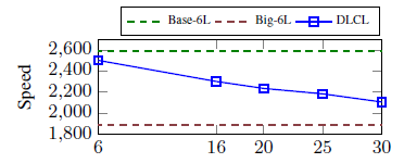
The proposed system with a 30-layer encoder is still faster than Transformer-Big.
3.5. Effect of Decoder Depth

Different from encoder, increasing the depth of decoder only yields a slight BLEU improvement.
3.6. Effect of DLCL

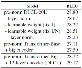
- Replacing learnable weights with constant weights: All-One (Wij=1) and Average (Wij=1/(i+1)) consistently hurt performance.
Making the weights learnable is important.
3.7. Weight Visualization

- The connections in the early layers are dense, but become sparse as the depth increases.
- Most of the large weight values concentrate on the right of the matrix, which indicates that the impact of the incoming layer is usually related to the distance between the outgoing layer, but the contribution to successive layers changes dynamically (one column).
Reference
[2019 ACL] [Pre-Norm Transformer]
Learning Deep Transformer Models for Machine Translation
Machine Translation
2014 [Seq2Seq] [RNN Encoder-Decoder] 2015 [Attention Decoder/RNNSearch] 2016 [GNMT] [ByteNet] [Deep-ED & Deep-Att] 2017 [ConvS2S] [Transformer] [MoE] [GMNMT] [CoVe] 2018 [Shaw NAACL’18] 2019 [AdaNorm] [GPT-2] [Pre-Norm Transformer] 2020 [Batch Augment, BA] [GPT-3] [T5] 2021 [ResMLP]
