Review — EfficientNetV2: Smaller Models and Faster Training

NAS and Scaling, Using New Ops Fused-MBConv

EfficientNetV2: Smaller Models and Faster Training
EfficientNetV2, by Google Research, Brain Team
2021 ICML, Over 120 Citations (Sik-Ho Tsang @ Medium)
Image Classification, EfficientNet

• A combination of training-aware neural architecture search (NAS) and scaling is used, to jointly optimize training speed and parameter efficiency.
• The models were searched from the search space enriched with new ops such as Fused-MBConv.
• EfficientNetV2 models train much faster than state-of-the-art models while being up to 6.8× smaller.

Outline

1. Understanding & Improving Training Efficiency of EfficientNetV1
2. Training-Aware NAS and Scaling
3. Progressive Learning
4. SOTA Comparison
5. Ablation Studies

1. Understanding & Improving Training Efficiency of EfficientNetV1

1.1. Training with Very Large Image Sizes is Slow

• EfficientNet’s large image size results in significant memory usage. Since the total memory on GPU/TPU is fixed, smaller batch size is used, which drastically slows down the training.

• FixRes can be used whereby using a smaller image size for training than for inference.
• As shown above, a smaller image size leads to fewer computations and enables large batch size, and thus improves training speed by up to 2.2× with slightly better accuracy.

1.2. Depthwise Convolutions are Slow in Early Layers but Effective in Later Stages

Structure of MBConv and Fused-MBConv

• Fused-MBConv is proposed in Google AI Blog: https://ai.googleblog.com/2019/08/efficientnet-edgetpu-creating.html

Fused-MBConv replaces the depthwise conv3×3 and expansion conv1×1 in MBConv with single regular conv3×3.

• Fused-MBConv gradually replaces the original MBConv in EfficientNet-B4 with Fused-MBConv.

When applied in early stage 1–3, Fused-MBConv can improve training speed with a small overhead on parameters and FLOPs.

• But if all blocks use Fused-MBConv (stage 1–7), then it significantly increases parameters and FLOPs while also slowing down the training.

1.3. Equally Scaling Up Every Stage is Sub-Optimal

• EfficientNet equally scales up all stages using a simple compound scaling rule. For example, when the depth coefficient is 2, then all stages in the networks would double the number of layers. However, these stages are not equally contributed to the training speed and parameter efficiency.
• In this paper, a non-uniform scaling strategy is used to gradually add more layers to later stages.
• In addition, EfficientNets aggressively scale up image size, leading to large memory consumption and slow training.
• To address this issue, the scaling rule is slightly modified and the maximum image size is restricted to a smaller value.

2. Training-Aware NAS and Scaling

2.1. NAS Search

• The neural architecture search (NAS) search space is similar to PNASNet.
• The design choices for convolutional operation types {MBConv, Fused-MBConv}, number of layers, kernel size {3×3, 5×5}, expansion ratio {1, 4, 6}.
• On the other hand, the search space size is reduced by:

1. removing unnecessary search options such as pooling skip ops, since they are never used in the original EfficientNets;
2. reusing the same channel sizes from the backbone as they are already searched in EfficientNets.

• Specifically, up to 1000 models are sampled and trained for about 10 epochs with reduced image size.
• The search reward combines the model accuracy A, the normalized training step time S, and the parameter size P, using a simple weighted product A×(S^w)×(P^v), where w=-0.07 and v=-0.05 are empirically determined.

EfficientNetV2-S Architecture

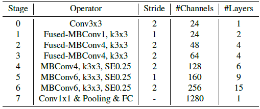
• The searched EfficientNetV2 has several major distinctions:

1. EfficientNetV2 extensively uses both MBConv and the newly added fused-MBConv in the early layers.
2. EfficientNetV2 prefers smaller expansion ratio for MBConv since smaller expansion ratios tend to have less memory access overhead.
3. Thirdly, EfficientNetV2 prefers smaller 3×3 kernel sizes, but it adds more layers to compensate for the reduced receptive field resulting from the smaller kernel size.
4. Lastly, EfficientNetV2 completely removes the last stride-1 stage in the original EfficientNet, perhaps due to its large parameter size and memory access overhead.

2.2. EfficientNetV2 Scaling

• EfficientNetV2-S is scaled up to obtain EfficientNetV2-M/L using similar compound scaling as EfficientNet, with a few additional optimizations:

1. The maximum inference image size is restricted to 480, as very large images often lead to expensive memory and training speed overhead;
2. As a heuristic, more layers are added gradually to later stages (e.g., stages 5 and 6) in order to increase the network capacity without adding much runtime overhead.

ImageNet accuracy and training step time on TPUv3

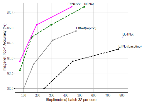
• With the training-aware NAS and scaling, the proposed EfficientNetV2 model train much faster than the other recent models.

3. Progressive Learning

The training process in the improved progressive learning

Progressive training settings for EfficientNetV2

ImageNet top-1 accuracy

• When image size is small, it has the best accuracy with weak augmentation; but for larger images, it performs better with stronger augmentation.
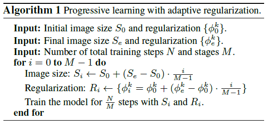
• It starts with small image size and weak regularization (epoch=1), and then gradually increases the learning difficulty with larger image sizes and stronger regularization: larger Dropout rate, RandAugment magnitude, and mixup ratio (e.g., epoch=300).
• Below shows the general algorithm:

Progressive learning with adaptive regularization

4. SOTA Comparison

4.1. ImageNet

EfficientNetV2 Performance Results on ImageNet

Model Size, FLOPs, and Inference Latency — Latency is measured with batch size 16 on V100 GPU

• Models marked with 21k are pre-trained on ImageNet21k with 13M images, and others are directly trained on ImageNet ILSVRC2012 with 1.28M images from scratch.

EfficientNetV2 models are significantly faster and achieves better accuracy and parameter efficiency than previous ConvNets and Transformers on ImageNet.

• In particular, EfficientNetV2-M achieves comparable accuracy to EfficientNet-B7 while training 11× faster using the same computing resources.
• EfficientNetV2 models also significantly outperform all recent RegNet and ResNeSt, in both accuracy and inference speed.
• The first figure at the top visualizes the results.

By pretraining on ImageNet21k (two days using 32 TPU cores), EfficientNetV2-L(21k) improves the top-1 accuracy by 1.5% (85.3% vs. 86.8%), using 2.5× fewer parameters and 3.6× fewer FLOPs, while running 6× — 7× faster in training and inference.

4.2. Transfer Learning Datasets

Transfer learning datasets

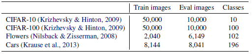
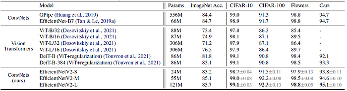
• Each model is finetuned with very few steps.
• EfficientNetV2 models outperform previous ConvNets and Vision Transformers for all these datasets.

e.g.: On CIFAR-100, EfficientNetV2-L achieves 0.6% better accuracy than prior GPipe/EfficientNets and 1.5% better accuracy than prior ViT/DeiT models. These results suggest that EfficientNetV2 also generalize well beyond ImageNet.

5. Ablation Studies

5.1. Performance with the Same Training

Comparison with the same training settings

• The performance comparison uses the same progressive learning settings.

EfficientNetV2 models still outperform EfficientNets by a large margin: EfficientNetV2-M reduces parameters by 17% and FLOPs by 37%, while running 4.1× faster in training and 3.1× faster in inference than EfficientNet-B7.

5.2. Scaling Down

Scaling down the model size

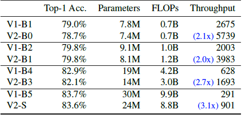
• Smaller models are compared by scaling down EfficientNetV2-S using EfficientNet compound scaling.
• All models are trained without progressive learning.

EfficientNetV2 (V2) models are generally faster while maintaining comparable parameter efficiency.

5.3. Progressive Learning for Different Networks

Progressive learning for ResNets and EfficientNets — (224) and (380) denote inference image size.

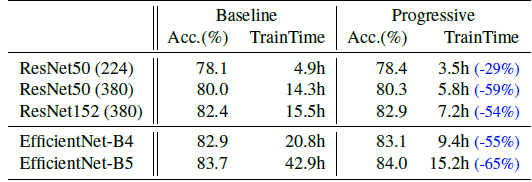
Progressive learning generally reduces the training time and meanwhile improves the accuracy for all different networks.

5.4. Importance of Adaptive Regularization

Adaptive regularization

Training curve comparison

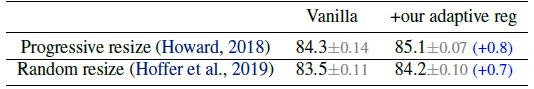
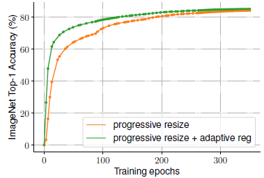
• Random resize: Because TPU needs to recompile the graph for each new size, here a image size is randomly sampled every eight epochs instead of every batch.

Adaptive regularization uses much smaller regularization for small images at the early training epochs, allowing models to converge faster and achieve better final accuracy.

Reference

[2021 ICML] [EfficientNetV2]
EfficientNetV2: Smaller Models and Faster Training

Image Classification

1989–2019 … 2020: [Random Erasing (RE)] [SAOL] [AdderNet] [FixEfficientNet] [BiT] [RandAugment]
2021: [Learned Resizer] [Vision Transformer, ViT] [ResNet Strikes Back] [DeiT] [EfficientNetV2]

My Other Previous Paper Readings