Review — SpineNet: Learning Scale-Permuted Backbone for Recognition and Localization

Using NAS for Scale-Permuted Intermediate Features & Cross-Scale Connections, Outperforms NAS-FPN in Object Detection, MnasNet in Image Classification

SpineNet Outperforms ResNet-FPN With Scale-Permuted Intermediate Features & Cross-Scale Connections

In this story, SpineNet: Learning Scale-Permuted Backbone for Recognition and Localization, (SpineNet), by Google Research, Brain Team, is reviewed.

Is the scale-decreased model a good backbone architecture design?

In this paper:

• SpineNet, is proposed, in which a backbone with scale-permuted intermediate features and cross-scale connections that is learned on an object detection task by Neural Architecture Search.

This is a paper in 2020 CVPR with over 50 citations. (Sik-Ho Tsang @ Medium)

Outline

1. SpineNet Overview
2. Resampling in Cross-Scale Connections
3. Scale-Permuted Model by Permuting ResNet
4. SpineNet Architectures
5. Object Detection Results
6. Image Classification Results

1. SpineNet Overview

Building scale-permuted network by permuting ResNet (Rectangle block represent bottleneck block and diamond block represent residual block. Output blocks are indicated by red border.)

1.1. Overview

1.1.1. ResNet-FPN

• (a) R50-FPN: ResNet-50 as backbone and FPN as detection network.
• ResNet is a scale-decreased model that the feature map dimensions are reduced for deeper layers/stages.
• Also, FPN selects pre-defined layers for feature map fusion for detection.

1.1.2. SpineNet

• (b) R23-SP30: The architecture of the proposed backbone model consists of a fixed stem network followed by a learned scale-permuted network, which obtains higher AP of 39.6%.
• (c) R0-SP53: All blocks are in a scale-permuted network, 40.7% AP.
• (d) SpineNet-49: Additional block adjustments (The selection of bottleneck or residual blocks) are included in the search space, 40.8% AP with fewer number of operations.
• A scale-permuted network is built with a list of building blocks {B1, B2, … , BN}.
• Each block Bk has an associated feature level Li. Feature maps in an Li block have a resolution of 1/(2^i) of the input resolution. The blocks in the same level have an identical architecture.
• Inspired by NAS-FPN, 5 output blocks are defined (Red Boundary Color Blocks), from L3 to L7 and a 1×1 convolution attached to each output block to produce multi-scale features P3 to P7 with the same feature dimension.
• The rest of the building blocks are used as intermediate blocks before the output blocks.

In Neural Architecture Search (NAS), the scale permutations for the intermediate and output blocks are first searched, then cross-scale connections between blocks are determined. The model are further improved by adding block adjustments in the search space.

1.2. Search Space

1.2.1. Scale permutations

• The orderings of blocks are important because a block can only connect to its parent blocks which have lower orderings.
• The search space of scale permutations are defined by permuting intermediate and output blocks respectively, resulting in a search space size of (N-5)!5!.
• The scale permutations are first determined before searching for the rest of the architecture.

1.2.2. Cross-Scale Connections

• Two input connections are used for each block.
• The parent blocks can be any block with a lower ordering or block from the stem network.
• Resampling spatial and feature dimensions is needed when connecting blocks in different feature levels.
• The search space has the size of:

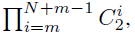
• where m is the number of candidate blocks in the stem network.

1.2.3. Block Adjustments

• The scale level and type of the block can be adjusted.
• The intermediate blocks can adjust levels by -{1, 0, 1, 2}, resulting in a search space size of 4^(N-5).
• All blocks are allowed to select one type between the two options {bottleneck block, residual block}, resulting in a search space size of 2N.

2. Resampling in Cross-Scale Connections

Resampling operations: Upper path need up-sample while lower path need down-sample to match the size of feature map in order for concatenation

• Cin and Cout are the input and output dimension of a block. For bottleneck block, Cin = Cout = 4C. For residual block, Cin = Cout = C.
• (Cout here is the output from the previous block, Cin is the input to the another block.)
• As it is important to keep the computational cost in resampling low, a scaling factor α (default value 0.5) is introduced.
• A nearest-neighbor interpolation for up-sampling or a stride-2 3×3 convolution (followed by stride-2 max poolings if necessary) for down-sampling feature map to match to the target resolution.
• Finally, a 1×1 convolution is applied to match feature dimension C to the target feature dimension Cin.
• Following FPN, element-wise addition is used.

3. Scale-Permuted Model by Permuting ResNet

• Scale-permuted models are built by permuting feature blocks in ResNet architecture.
• Small adaptation are made for scale-permuted models to generate multi-scale outputs by replacing one L5 block in ResNet with one L6 and one L7 blocks and the feature dimension is set to 256 for L5, L6, and L7 blocks.
• A family of models is generated that gradually shifts the model from the scale-decreased stem network to the scale-permuted network:

Number of blocks per level for stem and scale-permuted networks

• where use R[N]-SP[M] to indicate N feature layers in the handcrafted stem network and M feature layers in the learned scale-permuted network.
• Cross-scale connections only introduce small computation overhead.
• All models in the family, as shown in the above figure (b)-(d), have similar computation as ResNet-50.

4. SpineNet Architectures

4.1. SpineNet-49S/96/143/190

Increase model depth by block repeat. From left to right: blocks in SpineNet-49, SpineNet-96, and SpineNet-143

• Using ResNet-50 building blocks may not be an optimal choice. The optimal model may have different feature resolution and block type distributions. Additional block adjustments are included in the search space. The learnt model is called SpineNet-49, as in the above figure (d).
• 4 architectures are designed to support a wide range of latency-performance trade-offs.
• The models are denoted as SpineNet-49S/96/143/190:
• SpineNet-49S has the same architecture as SpineNet-49 but the feature dimensions in the entire network are scaled down uniformly by a factor of 0.65.
• SpineNet-96 doubles the model size by repeating each block Bk twice.
• SpineNet-143 and SpineNet-190 repeat each block 3 and 4 times to grow the model depth and adjust α in the resampling operation to 1.0. SpineNet-190 further scales up feature dimension uniformly by 1.3.

4.2. Object Detection (Some Details)

• The SpineNet architecture is learned with RetinaNet detector by simply replacing the default ResNet-FPN backbone model.
• For SpineNet-49S, 4 shared convolutional layers are used at feature dimension 128.
• For SpineNet-49/96/143, 4 shared convolutional layers are used at feature dimension 256.
• For SpineNet-190, subnets are scaled up by using 7 shared convolutional layers at feature dimension 512.
• In Mask R-CNN, For SpineNet-49S/49/96/143, 1 shared convolutional layers is used at feature dimension 256 for RPN, 4 shared convolutional layers at feature dimension 256 followed by a fully-connected layers of 1024 units for detection branch, and 4 shared convolutional layers at feature dimension 256 for mask branch.
• For SpineNet-49S, 128 feature dimension is used for convolutional layers in subnets.
• For SpineNet-190, detection subnets are scaled up by using 7 convolutional layers at feature dimension 384.

4.3. Image Classification (Some Details)

• P3 to P7 feature pyramid is used to construct the classification network.
• Specifically, the final feature map is generated by upsampling and averaging the feature maps:

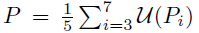
• where U(.) is the nearest-neighbor upsampling operation such that all feature maps have the same scale as the largest feature map P3.
• The standard global average pooling on P is applied to produce a 256-dimensional feature vector followed by a linear classifier with softmax for classification.

5. Object Detection Results

5.1. Importance of Cross-scale Connections

• For each block in the scale-permuted network of R0-SP53, cross-scale connections are damaged in three ways: (1) Removing the short-range connection; (2) Removing the long-range connection; (3) Removing both connections.
• (2) and (3) yield severer damage than (1), which is possibly because of short-range connection or sequential connection cannot effectively handle the frequent resolution changes.

5.2. ResNet-FPN vs SpineNet

Results comparisons between R50-FPN and scale-permuted models on COCO val2017

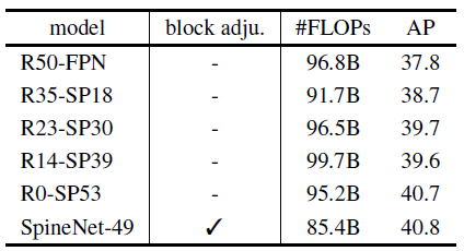
• The results in the above table support the claims that:

1. The scale-decreased backbone model is not a good design of backbone model for object detection;
2. Allocating computation on the proposed scale-permuted model yields higher performance.

Compared to the R50-FPN baseline, R0-SP53 uses similar building blocks and gains 2.9% AP with a learned scale permutations and cross-scale connections.

The SpineNet-49 model further improves efficiency by reducing FLOPs by 10% while achieving the same accuracy as R0-SP53 by adding scale and block type adjustments.

5.3. One-Stage Detector: RetinaNet

One-stage object detection results on COCO test-dev (+: Using More Advanced Training Protocol)

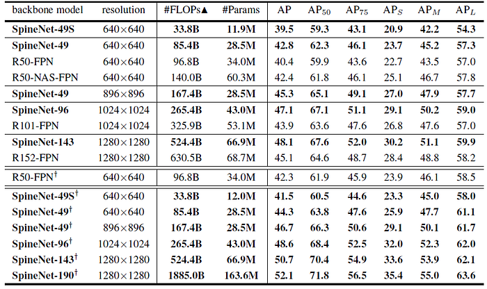
• SpineNet models outperform other popular detectors by large margins, such as ResNet-FPN, and NAS-FPN at various model sizes in both accuracy and efficiency.

The largest SpineNet-190 achieves 52.1% AP on single model object detection without test-time augmentation.

5.4. Two-Stage Detector: Mask R-CNN

Two-stage object detection and instance segmentation results

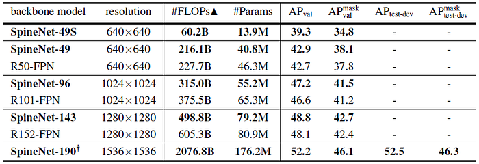
• Being consistent with RetinaNet results, SpineNet based models are able to achieve better AP and mask AP with smaller model size and less number of FLOPs.

5.5. Real-Time Object Detection

Inference latency of RetinaNet with SpineNet on a V100 GPU with NVIDIA TensorRT

• The SpineNet-49S and SpineNet-49 with RetinaNet run at 30+ fps with NVIDIA TensorRT on a V100 GPU.

5.6. Mobile-Size Object Detection

• MBConv blocks using the parametrization proposed in [37], which is the inverted bottleneck block with SE module, is used to build the block.
• Feature dimension {16, 24, 40, 80, 112, 112, 112}, expansion ratio 6, and kernel size 3×3 for L1 to L7 MBConv blocks.
• Each block in SpineNet-49 is replaced with the MBConv block at the corresponding level.
• SpineNet-49XS and SpineNet-49S are built by scaling the feature dimension of SpineNet-49 by 0.6 and 0.65 and setting the feature dimension in the box/class nets to 24 and 40 respectively.

Bulit with MBConv blocks, SpineNet-49XS/49S/49 use less computation but outperform MnasNet, MobileNetV2, and MobileNetV3 by 2–4% AP.

6. Image Classification Results

6.1. ImageNet & iNaturalist

Image classification results on ImageNet and iNaturalist

• Under the same setting, SpineNet’s performance is on par with ResNet on ImageNet but using much fewer FLOPs.
• iNaturalist-2017 is a challenging fine-grained classification dataset containing 579,184 training and 95,986 validation images from 5,089 classes.

On iNaturalist, SpineNet outperforms ResNet by a large margin of around 5%.

6.2. Further Improvements on SpineNet

Further improved SpineNet

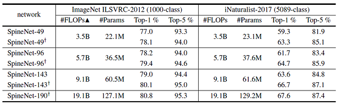
• SpineNet classification experiments using an improved training protocol by 1) adding stochastic depth, 2) replacing ReLU with swish activation and 3) using label smoothing of 0.1.

We can see that the improved training protocol yields around 1% Top-1 gain on ImageNet and 3–4% Top-1 gain on iNaturalist-2017.

Reference

[2020 CVPR] [SpineNet]
SpineNet: Learning Scale-Permuted Backbone for Recognition and Localization

Object Detection

2014–2017: …
2018: [YOLOv3] [Cascade R-CNN] [MegDet] [StairNet] [RefineDet] [CornerNet] [Pelee & PeleeNet]
2019: [DCNv2] [Rethinking ImageNet Pre-training] [GRF-DSOD & GRF-SSD] [CenterNet] [Grid R-CNN] [NAS-FPN] [ASFF] [Bag of Freebies]
2020: [EfficientDet] [CSPNet] [YOLOv4] [SpineNet]

My Other Previous Paper Readings