Review — SimSiam: Exploring Simple Siamese Representation Learning
Self-Supervised Learning Without the Use of Negative Sample Pairs, Large Batches, & Momentum Encoders
Exploring Simple Siamese Representation Learning
SimSiam, by Facebook AI Research (FAIR)
2021 CVPR, Over 500 Citations (Sik-Ho Tsang @ Medium)
Self-Supervised Learning, Unsupervised Learning, Representation Learning, Image Classification
- There are many different frameworks proposed for self-supervised learning, such as MoCo and SimCLR, yet with some constraints.
- A Simple Siamese network, SimSiam, is proposed, which can learn meaningful representations even using none of the following: (i) negative sample pairs, (ii) large batches, (iii) momentum encoders.
- A stop-gradient operation plays an essential role in preventing collapsing.
- (For quick read, please read 1, 2, 5.)
Outline
- SimSiam Framework
- Importance of Stop-Gradient
- Empirical Study for Other Settings
- Hypothesis
- SOTA Comparison
1. SimSiam Framework

1.1. Motivation
- In some prior arts, large amount of negative sample pairs which needs large batch, this leads to very high computational and memory requirement.
- To encounter this, some prior arts use momentum encoders as a workaround so that large batch is not needed.
SimSiam wants to remove all these to achieve a simple self-supervised learning framework.
1.2. Framework
- SimSiam takes as input two randomly augmented views x1 and x2 from an image x. The two views are processed by an encoder network f consisting of a backbone (e.g., ResNet) and a projection MLP head.
- The encoder f shares weights between the two views.
- A prediction MLP head, denoted as h, transforms the output of one view and matches it to the other view.
- Denoting the two output vectors:

- The negative cosine similarity is minimized:

- Following BYOL, the symmetric loss is used:

- This is defined for each image, and the total loss is averaged over all images. Its minimum possible value is −1.
An important component for SimSiam to work is a stop-gradient (stopgrad) operation:

- This means that z2 is treated as a constant in this term.
- Thus, the symmetric loss with:

- Here the encoder on x2 receives no gradient from z2 in the first term, but it receives gradients from p2 in the second term (and vice versa for x1).
1.3. Basic Settings
- ResNet-50 is used as the backbone encoder f.
- The batch size is 512 with 8 GPU used. Batch normalization (BN) is synchronized across devices.
- 100-epoch pretraining is performed.
- The projection MLP (in f) has BN applied to each fully-connected (fc) layer, including its output fc. Its output fc has no ReLU. The hidden fc is 2048-d. This MLP has 3 layers.
- The prediction MLP (h) has BN applied to its hidden fc layers. Its output fc does not have BN or ReLU. This MLP has 2 layers.
- The dimension of h’s input and output (z and p) is d=2048, and h’s hidden layer’s dimension is 512, making h a bottleneck structure.
2. Importance of Stop-Gradient Empirical Study

Left Plot: Without stop-gradient, the optimizer quickly finds a degenerated solution and reaches the minimum possible loss of −1.
- Middle Plot: shows the per-channel std of the ℓ2-normalized output, plotted as the averaged std over all channels. It shows that the degeneration is caused by collapsing.
With stop-gradient, the std value is near 1/√d. This indicates that the outputs do not collapse, and they are scattered on the unit hypersphere.
- Right Plot: With stop-gradient, the kNN monitor shows a steadily improving accuracy.
- Right Table: The linear evaluation result is shown. SimSiam achieves a nontrivial accuracy of 67.7%. Solely removing stop-gradient, the accuracy becomes 0.1%, which is the chance-level guess in ImageNet.
3. Empirical Study for Other Settings
The existence of the collapsing solutions implies that it is insufficient for SimSiam to prevent collapsing solely by the architecture designs (e.g., predictor, BN, ℓ2-norm). In other words, architecture designs do not prevent collapsing if stop-gradient is removed.
3.1. Predictor

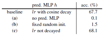
- (a): The model does not work if removing h (i.e. identity mapping). The loss becomes:

Using stop-gradient is equivalent to removing stop-gradient and scaling the loss by 1/2. Collapsing is observed.
3.2. Batch Size

Even a batch size of 128 or 64 performs decently, with a drop of 0.8% or 2.0% in accuracy. The results are similarly good when the batch size is from 256 to 2048.
- But but SimCLR and SwAV both require a large batch (e.g., 4096) to work well.
3.3. Batch Normalization (BN) on MLP Head

- Removing BN does not cause collapsing, but with 34.6% acc.
BN is helpful for optimization when it placed appropriately.
3.4. Similarity Function

- SimSiam also works with cross-entropy similarity though it may be suboptimal for this variant:

The cross-entropy variant can converge to a reasonable result without collapsing. This suggests that the collapsing prevention behavior is not just about the cosine similarity.
3.5. Symmetrization

The asymmetric variant achieves reasonable results. Symmetrization is helpful for boosting accuracy, but it is not related to collapse prevention.
4. Hypothesis
- In this section, authors try to use theoretical equations to explain the needs of stop-gradient and predictors.
4.1. Two Sub-Problems
SimSiam is an implementation of an Expectation-Maximization (EM) like algorithm. It implicitly involves two sets of variables, and solves two underlying sub-problems. The presence of stop-gradient is the consequence of introducing the extra set of variables.
- The loss function is:

- where F is a network parameterized by θ. T is the augmentation. x is an image. The expectation E[·] is over the distribution of images and augmentations. Mean square error is used for simplicity, which is equivalent to the cosine similarity if the vectors are ℓ2-normalized.
- Here, the predictor is not considered yet. As seen, η is introduced as another set of variables. And we consider solving:

- Here the problem is w.r.t. both θ and η. This formulation is analogous to k-means clustering, where θ is analogous to the clustering centers, and η is the representation of x.
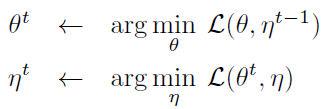
- Also analogous to k-means, the problem can be solved by an alternating algorithm, fixing one set of variables and solving for the other set. Formally, we can alternate between solving these two subproblems:

4.2. Solving for θ
- Here t is the index of alternation and “←” means assigning. One can use SGD to solve the sub-problem. The stop-gradient operation now become a natural consequence, because the gradient does not back-propagate to ηt−1 which is a constant in this problem.
4.3. Solving for η
- And the sub-problem for ηt, can be solved independently for each ηx. Now the problem is to minimize the below expectation for each image x:

- Due to the mean squared error, it is easy to solve it by:

- This indicates that ηx is assigned with the average representation of x over the distribution of augmentation.

4.4 One-Step Alternation
- SimSiam can be approximated by one-step alternation.
- First, the augmentation is sampled only once to approximate the first sub-problem, denoted as T′, and ignoring ET[·]:

- Inserting it into the second sub-problem, we have:

- Now θt is a constant in this sub-problem, and T′ implies another view due to its random nature.
This formulation exhibits the Siamese architecture. With one SGD step, it is a Siamese network naturally with stop-gradient applied.
4.5. Inclusion of Predictor
- By considering the predictor as well, the predictor h is expected to minimize:

- The optimal solution to h should satisfy for any image x:

- As in the approximation in 4.4, the expectation ET[·] is ignored. And in practice, it is unrealistic to actually compute the expectation ET. The usage of h may fill this gap.
4.6. k-step SGD for θ

- If k-step SGD within one epoch is considered for θ, “1-step” is equivalent to SimSiam, and “1-epoch” denotes the k steps required for one epoch.
All multi-step variants work well. The 10-/100-step variants even achieve better results than SimSiam.
5. SOTA Comparison
5.1. ImageNet Linear Evaluation

SimSiam is trained with a batch size of 256, using neither negative samples nor a momentum encoder. Despite it simplicity, SimSiam achieves competitive results. It has the highest accuracy among all methods under 100-epoch pre-training, though its gain of training longer is smaller.
- Also, it has better results than SimCLR in all cases.
5.2. Transfer Learning

- All methods are based on 200-epoch pre-training in ImageNet.
- SimSiam’s representations are transferable beyond the ImageNet task. All these methods are highly successful for transfer learning, they can surpass or be on par with the ImageNet supervised pre-training counterparts in all tasks. Siamese structure is a core factor for their general success.
5.3. Architecture Comparison

Reference
[2021 CVPR] [SimSiam]
Exploring Simple Siamese Representation Learning
Unsupervised/Self-Supervised Learning
1993 [de Sa NIPS’93] 2008–2010 [Stacked Denoising Autoencoders] 2014 [Exemplar-CNN] 2015 [Context Prediction] [Wang ICCV’15] 2016 [Context Encoders] [Colorization] [Jigsaw Puzzles] 2017 [L³-Net] [Split-Brain Auto] [Motion Masks] [Doersch ICCV’17] 2018 [RotNet/Image Rotations] [DeepCluster] [CPC/CPCv1] [Instance Discrimination] 2019 [Ye CVPR’19] 2020 [CMC] [MoCo] [CPCv2] [PIRL] [SimCLR] [MoCo v2] [iGPT] [BoWNet] [BYOL] [SimCLRv2] 2021 [MoCo v3] [SimSiam]
