[Review] ABN: Attention Branch Network for Visual Explanation (Image Classification)
Image Classification with Visual Explanation using Attention Map, Improved Accuracy for ResNet, Wide ResNet (WRN), DenseNet and ResNeXt

In this story, Attention Branch Network: Learning of Attention Mechanism for Visual Explanation, ABN, by Chubu University, is presented. In this paper:
- Attention Branch Network (ABN) is proposed, which extends a response-based visual explanation model by introducing a branch structure with an attention mechanism.
- ABN can be applicable to several image recognition tasks by introducing a branch for the attention mechanism and is trainable for visual explanation and image recognition in an end-to-end manner.
This is a paper in 2019 CVPR with over 60 citations. (Sik-Ho Tsang @ Medium)
Outline
- Attention Branch Network (ABN)
- ABN for Multi-Task Learning
- Experimental Results
1. Attention Branch Network (ABN)

- ABN consists of three modules: feature extractor, attention branch, and perception branch, as shown above.
- ABN is based on a baseline model such as VGGNet and ResNet.
- The attention branch is constructed after feature extractor on the basis of the CAM.
1.1. Attention Branch
- CAM has a K×3×3 convolution layer, GAP, fully-connected layer, and softmax as the last layers, as shown above, where K is the number of categories.
- Each feature map there represents the attention location for each class.
- When CAM visualizes the attention map of each class, an attention map is generated by multiplying the weighted sum of the K×h×w feature map by the weight at the last fully-connected layer.
- Instead of using fully-connected layer, the attention branch generates an attention map from the K×h×w feature map.
- These feature maps are convolved by a 1×1×1 convolution layer, then normalized by the sigmoid function.
1.2. Perception Branch
- The perception branch outputs the final probability of each class by receiving the attention and feature maps from the feature extractor.
- It uses one of the below equations for the attention mechanism:

- where gc(xi) is the feature map at the feature extractor, M(xi) is an attention map, and g’c(xi) is the output of the attention mechanism.
- The first equation is simply a dot-product between the attention and feature maps at a specific channel c.
- In contrast, the second equation can highlight the feature map at the peak of the attention map while preventing the lower value region of the attention map from degrading to zero.
- (This part is similar to Residual Attention Network. If interested, please feel free to read it.)
1.3. Training
- The training loss function L(xi) is a simple sum of losses at both branches:
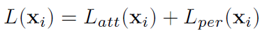
- where Latt(xi) denotes training loss at the attention branch with an input sample xi, and Lper(xi) denotes training loss at the perception branch.
2. ABN for Multi-Task Learning

- In image classification, the relation between the numbers of inputs and recognition tasks is one-to-one. The one-to-one relation can be focused on the specific target location using a single attention map
- In contrast, the relation between the numbers of inputs and recognition tasks of multi-task learning is one-to-many.
- One-to-many relation cannot be focused on multiple target locations using a single attention map. To address this issue, ABN generates multiple attention maps for each task by introducing multi-task learning to the attention and perception branches.
- ResNet with multi-task learning is used as baseline.
- First, a feature map at residual block 4 is convoluted by the T×1×1 convolution layer, and the T×14×14 feature map is output, where T is the number of tasks.
- The probability score during a specific task {t|1,…,T} is output by applying the 14×14 feature map at specific task t to GAP and the sigmoid.
- This probability matrix of each task on the perception branch consists of T×2 components defined two categories classification for each task.
3. Experimental Results
3.1. Classification

- g(x) is conventional ResNet.
- Attention mechanism g(x)⋅(1 +M(x)) is slightly more accurate than attention mechanism g(x)⋅M(x).
- Thus, g(x)⋅(1 +M(x)) is used in the below experiments.

- Accuracies of ResNet, Wide ResNet (WRN), DenseNet and ResNeXt are improved by introducing ABN.
- On CIFAR10, ResNet and DenseNet with ABNs decrease the top-1 errors from 6.43% to 4.91% and 4.51% to 4.17%, respectively.
- Additionally, all ResNet models are decrease the top-1 errors by more 0.6% on CIFAR100.
- On ImageNet, the performance of CAM slightly decreased with a specific baseline model because of the removal of the fully-connected layers and adding a GAP.
- On the other hand, ABN outperforms conventional VGGNet and CAM and performs better than conventional ResNet and CAM.
- By introducing the SE modules to ResNet152, SENet reduces the top-1 errors from 22.19% to 21.90%.
- However, ABN reduces the top-1 errors from 22.19% to 21.37%, indicating that ABN is more accurate than SENet.
- Moreover, ABN can introduce the SENet in parallel. SENet with ABN reduces the top-1 errors from 22.19% to 20.77% compared to the ResNet152.
3.2. Visualization

- For the third column, this original image is a typical example because multiple objects, such as “Seat belt” and “Australian terrier”, are included. In this case, Grad-CAM (conventional ResNet152) and CAM failes, but ABN performs well.
- Therefore, this attention map can focus on a specific region when multiple objects are in an image.
3.3. Fine-Grained Recognition
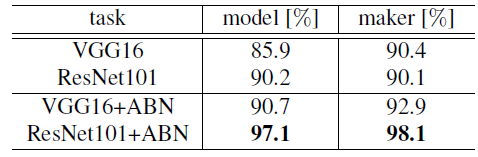
- The comprehensive cars (CompCars) dataset has 36,451 training images and 15,626 testing images with 432 car models and 75 makers.
- The car model recognition accuracy of ABN improves by 4.9% and 6.2 % with VGG16 and ResNet101, respectively.
- Moreover, maker recognition accuracy improves by 2.0 and 7.5 %, respectively.
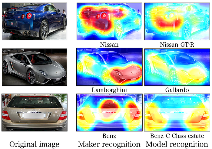
Training and testing images are the same for car model and maker recognition. The proposed attention maps differ depending on the recognition task.
4.4. Multi-Task Learning
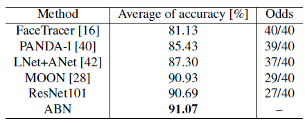
- Multiple facial attributes recognition is evaluated using the CelebA dataset, which consists of 202,599 images (182,637 training images and 19,962 testing images) with 40 facial attribute labels.
- ABN outperforms all conventional methods regarding the average recognition rate and number of facial attribute tasks.
- When comparing ResNet101 and ABN, ABN is 0.38% more accurate. Moreover, the accuracy of 27 facial tasks is improved. ABN also performs better than conventional facial attribute recognition models.

- The above figure shows the attention map of ABN on CelebA dataset. These attention maps highlights the specific locations such as mouth, eyes, beard, and hair. These highlight locations correspond to the specific facial task.
Reference
[2019 CVPR] [ABN]
Attention Branch Network: Learning of Attention Mechanism for Visual Explanation
Image Classification
1989–1998: [LeNet]
2012–2014: [AlexNet & CaffeNet] [Dropout] [Maxout] [NIN] [ZFNet] [SPPNet]
2015: [VGGNet] [Highway] [PReLU-Net] [STN] [DeepImage] [GoogLeNet / Inception-v1] [BN-Inception / Inception-v2]
2016: [SqueezeNet] [Inception-v3] [ResNet] [Pre-Activation ResNet] [RiR] [Stochastic Depth] [WRN] [Trimps-Soushen]
2017: [Inception-v4] [Xception] [MobileNetV1] [Shake-Shake] [Cutout] [FractalNet] [PolyNet] [ResNeXt] [DenseNet] [PyramidNet] [DRN] [DPN] [Residual Attention Network] [IGCNet / IGCV1] [Deep Roots]
2018: [RoR] [DMRNet / DFN-MR] [MSDNet] [ShuffleNet V1] [SENet] [NASNet] [MobileNetV2] [CondenseNet] [IGCV2] [IGCV3] [FishNet] [SqueezeNext] [ENAS] [PNASNet] [ShuffleNet V2] [BAM] [CBAM] [MorphNet] [NetAdapt] [mixup] [DropBlock]
2019: [ResNet-38] [AmoebaNet] [ESPNetv2] [MnasNet] [Single-Path NAS] [DARTS] [ProxylessNAS] [MobileNetV3] [FBNet] [ShakeDrop] [CutMix] [MixConv] [EfficientNet] [ABN]
2020: [Random Erasing (RE)]