Review — CB Loss: Class-Balanced Loss Based on Effective Number of Samples (Image Classification)

Using the Effective Number of Samples for Each Class to Re-Balance the Loss, Outperforms Focal Loss in RetinaNet

Published in

Nerd For Tech

7 min readMar 7, 2021

In this paper, Class-Balanced Loss Based on Effective Number of Samples, (CB Loss), by Cornell University, Cornell Tech, Google Brain, and Alphabet Inc., is reviewed. In this paper:

A re-weighting scheme is designed that uses the effective number of samples for each class to re-balance the loss, called class-balanced loss.

This is a paper in 2019 CVPR over 200 citations. (Sik-Ho Tsang @ Medium)

Outline

Class Imbalance Problem
Effective Number of Samples
Class-Balanced Loss (CB Loss)
Experimental Results

1. Class Imbalance Problem

**Two classes, one from the head and one from the tail of a long-tailed dataset (iNaturalist 2017 Dataset)**

Suppose there are classes that arm imbalanced as above.
Head: For the class with small indices, these classes have the larger number of samples.
Tail: For the class with large index, these classes have the smaller number of samples.
Black Solid Line: Models directly trained on these samples are biased toward dominant classes.
Red Dashed Line: Re-weighting the loss by inverse class frequency may yield poor performance on real-world data with high class imbalance.
Blue Dashed Line: A class-balanced term is designed to re-weight the loss by inverse effective number of samples.

2. Effective Number of Samples

2.1. Definition

**Information Overlap Among Data, Left: Feature Space S, Middle: Unit Volume of 1 Sample Data, Right: Information Overlapping Among Data**

Intuitively, the more data, the better. However, since there is information overlap among data, as the number of samples increases, the marginal benefit a model can extract from the data diminishes.

Left: Given a class, denote the set of all possible data in the feature space of this class as S. Assume the volume of S is N and N ≥ 1.
Middle: Each sample in a subset of S has the unit volume of 1 and may overlap with other samples.
Right: Each subset is randomly sampled from S to cover the entire set of S. The more data is being sampled, the better the coverage of S is.
The expected total volume of sampled data increases as the number of samples increases and is bounded by N.

Therefore, the effective number of samples is defined as the expected volume of samples.

The idea is to capture the diminishing marginal benefits by using more data points of a class.
Due to intrinsic similarities among real-world data, as the number of samples grows, it is highly possible that a newly added sample is a near-duplicate of existing samples.
In addition, CNNs are trained with heavy data augmentations, all augmented examples are also considered as same with the original example.
For a class, N can be viewed as the number of unique prototypes.

2.2. Mathematical Formulation

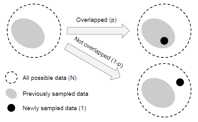
**New Sampled Data is Either Overlapped or Not Overlapped with Previously Sampled Data**

Denote the effective number (expected volume) of samples as En.
To simplify the problem, the situation of partial overlapping is not considered.
That is, a newly sampled data point can only interact with previously sampled data in two ways: either entirely inside the set of previously sampled data with the probability of p or entirely outside with the probability of 1-p.
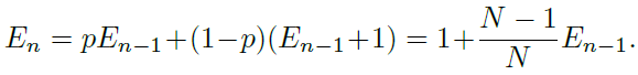
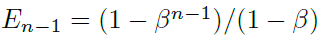
Proposition (Effective Number): En = (1−β^n)/(1−β), where
β = (N− 1)/N. This proposition is proved by mathematical induction.
When E1 = 1, there is no overlapping. E1 = (1−β^1)/(1−β) = 1 holds.
Consider there are previously sampled n−1 examples and are about to sample the nth example. Now the expected volume of previously sampled data is En−1 and the newly sampled data point has the probability of p = E(n−1)/N to be overlapped with previous samples. Therefore, the expected volume after sampling nth example is:

With:

We got:

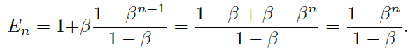
The above proposition shows that the effective number of samples is an exponential function of n.
The hyperparameter β ∈ [0, 1) controls how fast En grows as n increases.

3. Class-Balanced Loss (CB Loss)

The class-balanced (CB) loss is written as:

where ny is the number of samples in the ground-truth class y.
β = 0 corresponds to no re-weighting and β → 1 corresponds to re-weighing by inverse class frequency.

The proposed novel concept of effective number of samples enables us to use a hyperparameter β to smoothly adjust the class-balanced term between no re-weighting and re-weighing by inverse class frequency.

The proposed class-balanced term is model-agnostic and loss-agnostic in the sense that it is independent to the choice of loss function L and predicted class probabilities p.

3.1. Class-Balanced Softmax Cross-Entropy Loss

Given a sample with class label y, the softmax cross-entropy (CE) loss for this sample is written as:

Suppose class y has ny training samples, the class-balanced (CB) softmax cross-entropy loss is:

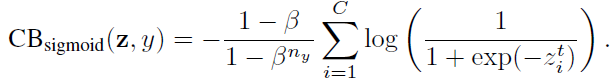
3.2. Class-Balanced Sigmoid Cross-Entropy Loss

When using sigmoid function for multi-class problem, each output ode of the network is performing a one-vs-all classification to predict the probability of the target class over the rest of classes.
In this case, Sigmoid doesn’t assume the mutual exclusiveness among classes.
Since each class is considered independent and has its own predictor, sigmoid unifies single-label classification with multi-label prediction. This is a nice property to have since real-world data often has more than one semantic label.
The sigmoid cross-entropy (CE) loss can be written as:

The class-balanced (CB) sigmoid cross-entropy loss is:

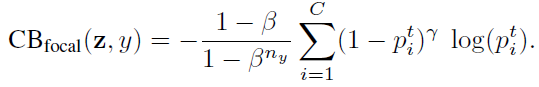
3.3. Class-Balanced Focal Loss

The focal loss (FL) proposed in RetinaNet, reduce the relative loss for well-classified samples and focus on difficult samples:

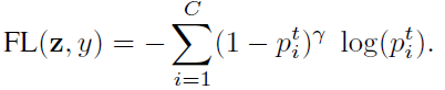
(For more details, if interested, please feel free to read RetinaNet.)
The class-balanced (CB) Focal Loss is:

4. Experimental Results

4.1. Datasets

**Datasets that are used to evaluate the effectiveness of class-balanced loss**

5 long-tailed versions of both CIFAR-10 and CIFAR-100 with imbalance factors of 10, 20, 50, 100 and 200 respectively, are tried.
iNaturalist and ILSVRC are class imbalance in nature.

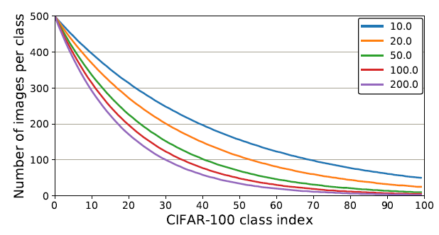
**Number of training samples per class in artificially created long-tailed CIFAR-100 datasets with different imbalance factors.**

The above shows the number of images per class with different imbalance factors.

4.2. CIFAR Datasets

**Classification error rate of** **ResNet-32 trained with different loss functions on long-tailed CIFAR-10 and CIFAR-100 Test Sets**

The search space of hyperparameters is {softmax, sigmoid, focal} for loss type, β ∈ {0.9, 0.99, 0.999, 0.9999}, and γ ∈ {0.5, 1.0, 2.0} for Focal Loss.
The best β is 0.9999 on CIFAR-10 unanimously.
But on CIFAR-100, datasets with different imbalance factors tend to have different and smaller optimal β.

**Classification error rate when trained with and without the class-balanced term.**

On CIFAR-10, when re-weighting based on β = 0.9999, the effective number of samples is close to the number of samples. This means the best re-weighting strategy on CIFAR-10 is similar with re-weighting by inverse class frequency.
On CIFAR-100, the poor performance of using larger β suggests that re-weighting by inverse class frequency is not a wise choice. A smaller β is needed that has smoother weights across classes.
For example, the number of unique prototypes of a specific bird species should be smaller than the number of unique prototypes of a generic bird class. Since classes in CIFAR-100 are more fine-grained than CIFAR-10, CIFAR-100 have smaller N compared with CIFAR-10.

4.3. Large-Scale Datasets

**Top-1 and Top-5 Classification error rate on large-scale datasets trained with different loss functions on validation set of all datasets**

The class-balanced Focal Loss is used since it has more flexibility and it is found that β = 0.999 and γ = 0.5 yield reasonably good performance on all datasets.
Notably, ResNet-50 is able to achieve comparable performance with ResNet-152 on iNaturalist and ResNet-101 on ILSVRC 2012 when using class-balanced Focal Loss to replace softmax cross-entropy loss.