Review — Swin Transformer V2: Scaling Up Capacity and Resolution
Swin V2, Improves Swin V1

Swin Transformer V2: Scaling Up Capacity and Resolution,
Swin Transformer V2, by Microsoft Research Asia,
2022 CVPR, Over 300 Citations (Sik-Ho Tsang @ Medium)Image Classification
1989 … 2022 [ConvNeXt] [PVTv2] [ViT-G] [AS-MLP] [ResTv2] [CSWin Transformer] [Pale Transformer] [Sparse MLP] [MViTv2] [S²-MLP] [CycleMLP] [MobileOne] [GC ViT] [VAN] [ACMix] [CVNets] [MobileViT] [RepMLP] [RepLKNet] [ParNet] [MetaFormer, PoolFormer] 2023 [Vision Permutator (ViP)]
==== My Other Paper Readings Are Also Over Here ====
- Three main techniques are proposed:
- A residual-post-norm method combined with cosine attention to improve training stability.
- A log-spaced continuous position bias method to effectively transfer models pre-trained using low-resolution images to downstream tasks with high-resolution inputs
- A self-supervised pretraining method, SimMIM, is used to reduce the needs of vast labeled images.
- Finally, a 3 billion-parameter Swin Transformer V2 model can be trained, which is the largest dense vision model to date, and makes it capable of training with images of up to 1536×1536 resolution.
Outline
- Swin V2 Residual-Post Norm
- Swin V2 Scaled Cosine Attention
- Swin V2 Scaling Up Window Resolution
- Swin V2 Self-Supervised Pretraining Using SimMIM
- Implementation to Save GPU Memory
- Model Variants
- Experimental Results
1. Swin V2 Residual-Post Norm
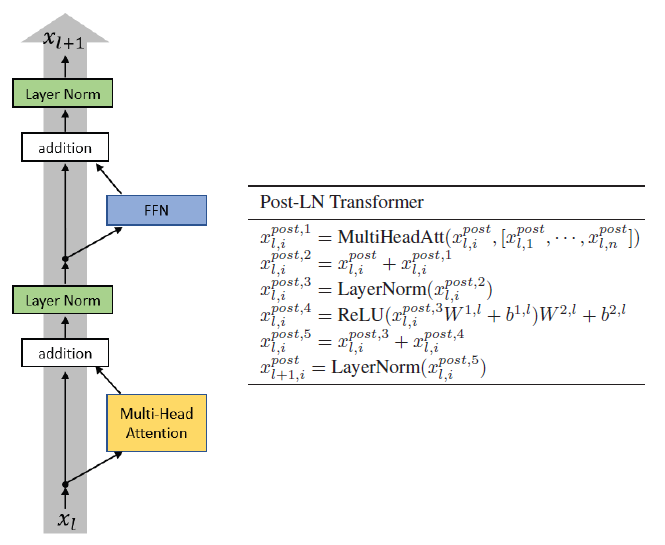
1.1. Original Pre Norm
1.2. Swin V2 Post Norm

- In Swin V2, Residual post normalization approach (Post) is proposed

The activation amplitudes (Post) are much milder than in the original pre-normalization configuration (Pre).

- When scaling up the original Swin V1 from small size to large size, the activation values at deeper layers increase dramatically. The discrepancy between layers with the highest and the lowest amplitudes has reached an extreme value of 10⁴.
When scaling it up further to a huge size (658 million parameters), it cannot complete the training.
2. Swin V2 Scaled Cosine Attention
2.1. Original Self-Attention
- In the original self-attention computation, the similarity terms of the pixel pairs are computed as a dot product of the query and key vectors, QK^T.

- When this approach is used in large visual models, the learnt attention maps of some blocks and heads are frequently dominated by a few pixel pairs, especially in the res-post-norm configuration.
2.2. Swin V2 Scaled Cosine Attention
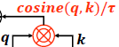
- In Swin V2, to ease this issue, a scaled cosine attention approach is proposed, which computes the attention logit of a pixel pair i and j by a scaled cosine function:
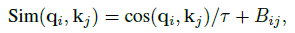
- where Bij is the relative position bias between pixel i and j. τ is a learnable scalar, non-shared across heads and layers. τ is set larger than 0.01.
The cosine function is naturally normalized, and thus can have milder attention values.
3. Scaling Up Window Resolution
3.1. Original Parameterized Relative Position Bias
- The relative positions along each axis are within the range of [-M+1, M+1] and the relative position bias is parameterized as a bias matrix ^B.
- When transferring across different window sizes, the learnt relative position bias matrix in pre-training is used to initialize the bias matrix of a different size in fine-tuning by bi-cubic interpolation.
3.2. Swin V2 Linear-Spaced Continuous Position Bias (CPB)

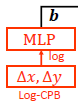
- The continuous position bias (CPB) approach adopts a small meta network on the relative coordinates:
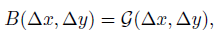
- where G is a small network, e.g., a 2-layer MLP with a ReLU activation in between by default. (It is the “MLP” in the figure of Swin V2 block.)
- The meta network G generates bias values for arbitrary relative coordinates, and thus can be naturally transferred to fine-tuning tasks with arbitrarily varying window sizes.
- In inference, the bias values at each relative position can be pre-computed and stored as model parameters.
3.3. Swin V2 Log-Spaced CPB
- When transferring across largely varying window sizes, a large portion of the relative coordinate range needs to be extrapolated.
- To ease this issue, log-spaced coordinates are used instead of the original linear-spaced ones:
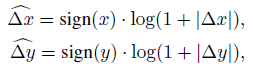
- where Δx, Δy and ^Δx, ^Δy are the linear-scaled and log-spaced coordinates, respectively.
e.g.: Transferring from a pre-trained 8×8 window size to a fine-tuned 16×16 window size, the input coordinate range will be from [-7, 7]×[-7, 7] to [-15, 15]×[-15, 15]. The extrapolation ratio is 8/7=1.14 of the original range.
Using log-spaced coordinates, the input range will be from [-2.079, 2.079]×[2.079, 2.079] to [-2.773, 2.773]×[-2.773, 2.773]. The extrapolation ratio is 0.33× which is 4 times smaller.

The bias matrices learnt by two CPB approaches are more smoothly than that learnt by P-RPE parameterized relative position bias).
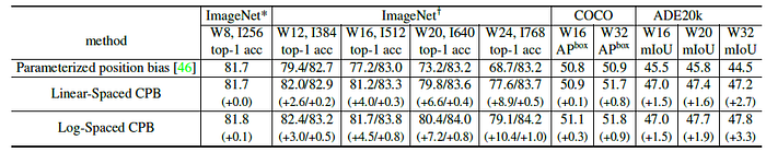
The log-spaced CPB approach performs best, particularly when transferred to larger window sizes.
4. Self-Supervised Pretraining Using SimMIM
- Self-supervised SimMIM [72], is used to alleviate the demands on labelled data. (Since SimMIM is another concurrent 2022 CVPR paper, I will have another story to talk about it.)
By this approach, a powerful Swin V2 of 3 billion parameters, is successfully trained, which achieves state-of-the-art (SOTA) on 4 representative visual benchmarks, by using only 70 million labelled images (1/40 of that in JFT-3B).
5. Implementation to Save GPU Memory
- Another issue lies in the unaffordable GPU memory consumption with a regular implementation when both the capacity and resolution are large.
With below implementations, a 3B model is managed to be trained using the Nvidia A100–40G GPUs for COCO object detection with an input image resolution of 1536×1536 and Kinetics-400 action classification with an input resolution of 320×320×8.
5.1. Zero-Redundancy Optimizer (ZeRO) [54]
- A model of 3 billion parameters will consume 48G GPU memory when an AdamW optimizer and fp32 weights/states are used.
With a ZeRO optimizer, the model parameters and the corresponding optimization states are split and distributed to multiple GPUs, which significantly reduces memory consumption.
5.2. Activation Check-Pointing [12]
- Feature maps in the Transformer layers also consume a lot of GPU memory, which can create bottlenecks when image and window resolutions are high.
The activation checkpointing technology can significantly reduce the memory consumption, while the training speed is up to 30% slower.
5.3. Sequential Self-Attention Computation
- For an image of 1536×1536 resolution with a window size of 32×32, regular A100 GPUs (40GB memory) are still unaffordable for self-attention computation.
Self-attention computation are implemented sequentially, instead of using the previous batch computation approach. This optimization is applied to the layers in the first two stages and has little impact on the overall training speed.
6. Swin V2 Model Variants
- 4 configurations of Swin Transformer V2 are used, which maintain the stage, block, and channel settings of the original Swin V1:
- SwinV2-T: C=96, #. block = {2, 2, 6, 2}
- SwinV2-S/B/L: C=96=128=192, #.block={2, 2, 18, 2}
- It is further scaled up to its huge size and giant size, with 658 million parameters and 3 billion parameters, respectively:
- SwinV2-H: C=352, #. block = {2, 2, 18, 2}
- SwinV2-G: C=512, #. block = {2, 2, 42, 4}
- For SwinV2-H and SwinV2-G, an additional normalization layer is added on the main branch every 6 layers.
7. Experimental Results
7.1. Image Classification

- SwinV2-G is the largest dense vision model to present.
It achieves a top-1 accuracy of 84.0% on the ImageNet V2 benchmark, which is +0.7% higher than previous best one (83.3%).
The accuracy on ImageNet-1K V1 is marginally lower (90.17% vs 90.88%). The performance difference might come from different degrees of dataset overtuning [55]. Also note we employ much less training iterations and lower image resolutions.
7.2. Downstream Tasks

- COCO Object Detection: SwinV2-G achieves 63.1/54.4 box/max AP on COCO test-dev, which is +1.8/1.4 higher than previous best number (61.3/53.0 by [74]). SwinV2-G can use a different window size at test to additionally benefit, probably attributed to the effective Log-spaced CPB approach.
- ADE20K Semantic Segmentation: SwinV2-G achieves 59.9 mIoU on ADE20K val set, +1.5 higher than the previous best number (58.4 by [4]). Using a larger window size at test time can additionally bring +0.2 gains, probably attributed to the effective Log-spaced CPB approach.
- Kinetics-400 Action Classification: SwinV2-G 86.8% top-1 accuracy, +1.4% higher than previous best number [57]. Again, using a larger window size at test time can also bring additional benefits of +0.2%.
7.3. Ablation Study

- Left: Both res-post-norm and cosine attention techniques improve the accuracy at all the tiny, small and base size, and the overall improvements are +0.2%, +0.4% and +0.5% respectively.
- Top Right: The proposed norm outperforms other normalization methods.
- Bottom Right: Log-CPB performs consistently better than the parameterized position bias approach used in Swin V1.


![Understanding the [CLS] Token in BERT: A Comprehensive Guide](https://miro.medium.com/v2/resize:fit:679/0*uHKOsv_avk-tKDCZ.png)